We will start with a blank jupyter notebook and we will define and train a neural net while showcasing everything that goes on under the hood. So we will be building this autograd (short for automatic gradient, hence the name zdravkograd) and basically it implements backpropogation. Backpropogration is essentially this algorithm that allows you to efficiently evaluate the gradient of some kind of loss function with respect to the weights of a neural network. This will allow us to iteratively tune the weights of this neural network to minimise the loss function and therefore improve the accuracy of the network. Backpropogation is the mathematic core of any modern deep neural network library, like PyTorch for example.
Neural networks are just a mathematical expression, they take input data as an input as well as the weight data as an input and the output of this mathematical expression are the network's predictions of the neural net (or the loss function).
Running through this project is a much better way to understand and learn about backpropogration, the chain rule and training neural networks rather than going straight into using something like PyTorch, it breaks the unnecessary things out of PyTorch like Tensors and will give me a much better understanding of what really happens in terms of how a neural net is trained at the most fundamental level.
This project is basically all you need in order to train neural networks, everything else added on top or after this is purely just for efficiency. At the end we will end up with essentially two python files: engine.py (that knows nothing about neural nets really) and nn.py. nn.py is the neural network library built on top of the autograd engine and its quite simple actually. We will be defining what a Neuron is and then what a Layer of neurons is and then define what a multilayer perceptron (MLP) which is just a sequence of layers of neurons. Broken down that's all you need to understand neural network training, everything else is just efficiency. Ok so let's start.
The first thing we need to understand very well is what a derivative is and what information it gives you. So let's start with some basic imports that we will need throughout this whole project:
import math
import numpy as np
import matplotlib.pyplot as plt
%matplotlib inline
And now lets also define this scalar value function f(x):
def f(x):
    return 3*x**2 - 4*x + 5
We can now call this function with say 3, f(3.0) and we will get 20.0 back.
Now we can also plot this function to get a sense for its shape and given its mathematical expression you should be able to tell that its going to be a parabola, its quadratic.
So lets just create a set of scalar values that we can feed in using arage from negative 5 to 5 in steps of 0.25: xs = np.arange(-5, 5, 0.25), and if we print that out we now have:
array([-5.  , -4.75, -4.5 , -4.25, -4.  , -3.75, -3.5 , -3.25, -3.  ,
       -2.75, -2.5 , -2.25, -2.  , -1.75, -1.5 , -1.25, -1.  , -0.75,
       -0.5 , -0.25,  0.  ,  0.25,  0.5 ,  0.75,  1.  ,  1.25,  1.5 ,
        1.75,  2.  ,  2.25,  2.5 ,  2.75,  3.  ,  3.25,  3.5 ,  3.75,
        4.  ,  4.25,  4.5 ,  4.75])
Now we can call our function on these values with ys = f(xs), and the ys look like this:
array([100.    ,  91.6875,  83.75  ,  76.1875,  69.    ,  62.1875,
        55.75  ,  49.6875,  44.    ,  38.6875,  33.75  ,  29.1875,
        25.    ,  21.1875,  17.75  ,  14.6875,  12.    ,   9.6875,
         7.75  ,   6.1875,   5.    ,   4.1875,   3.75  ,   3.6875,
         4.    ,   4.6875,   5.75  ,   7.1875,   9.    ,  11.1875,
        13.75  ,  16.6875,  20.    ,  23.6875,  27.75  ,  32.1875,
        37.    ,  42.1875,  47.75  ,  53.6875])
We can now plot this using matplotlib using plt.plot(xs, ys) and we will get this:
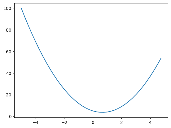
Previously we inputted 3.0 and we got 20.0 back which matches with our graph.
So now, let's think about what is the derivative of this function at any single input x? I hope this is something you know because its really easy, you should have learnt this in math class. Here we are not going to go and do this whole math stuff but you should know it. Instead lets look at the definition of what a derivative really is and what does it tell you about the function.
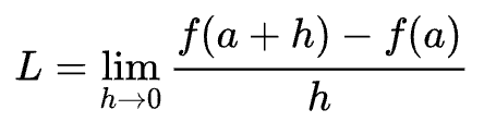
You should recognise this image, it tells us that a derivative is the limit as h goes to 0 of f(a + h) - f(a) all over h. This tells us that if you slightly bump up a (at whatever point you are interested in) by some small amount h how does the function respond, with what sensitivity does it respond, what is the slope at that point? Does the function go up or does it go down and by how much? And that is the slope of that function at that point.
So now if we use that in our code, lets take a very small amount of h, h = 0.001, and again lets say we are interested in the point at x = 3.0 and we pass it inf(x), which we know is 20. So now if we slightly nudge the point by h, f(x + h), so we are slightly nudging x in a positive direction, how will the function respond? If we go back and look at the graph we will expect f(x + h) to be greater of course. And if we calculate that:
h = 0.001
x = 3.0
f(x + h)
We get: 20.014003000000002, which is what we expected, its slightly more positive, and now by how much is telling you the strength of that slope. And if we do:
h = 0.001
x = 3.0
f(x + h) - f(x)
We can get that number showing us by how much the function responded: 0.01400300000000243, now we just have to normalise by the run (remember the rise over the run), so lets divide it all by h:
h = 0.001
x = 3.0
(f(x + h) - f(x)) / h
That gives us 14.00300000000243, this is the numerical approximation of the slope (because we have to make h very very small to converge to the exact amount). We do have to be careful here though because if you do too many zeros:
h = 0.0000000000000001
x = 3.0
(f(x + h) - f(x)) / h
At some point we will get the incorrect answer of 0.0 because we are using floating point arithmetic and the representations of all these numbers in computer memory is finite and at some point we get into this trouble.
Ok, so we have found that at 3.0 the slope is 14. And you can prove that by taking our expression, 3x^2 - 4x + 5 and differentiating it to get 6x - 4 and if you plug 3 in you get: 18 - 4 which is 14, nice.
Now lets take a look at a bit more of a complex case.
a = 2.0
b = -3.0
c = 10.0
d = a*b + c
print(d)
We now have d that is a function of three scalar inputs a, b, and c. If we print d now we get 4. Let's now look at the derivative of d with respect to a, b and c and then think through what this derivative is telling us. To do this again we will have some very small value of h: h = 0.0001 and we will fix these inputs at the numbers you see above. So this is the point a, b, c where we will be evaluating the derivative of d with respect to all a, b and c.
h = 0.0001

a = 2.0
b = -3.0
c = 10.0

d1 = a*b + c
a += h
d2 = a*b + c

print('d1 = ', d1)
print('d2 = ', d2)
print('slope = ', (d2 - d1) / h)
Now if we run this what do we expect to see, well we know that d1 is 4.0, in d2 we are bumping a up by h. So if we just think about this a little, what do we expect d2 to be? a here will now be slightly more positive but b is a negative number so that means that we will be adding less to d because it a*b will be a lower number. So we are expecting d2 to go lower. If I run this without the last print we get
d1 =  4.0
d2 =  3.999699999999999
Yeah, ok, as we expected, we went from 4 to 3.999699999999999. This tells us that the slope will be negative, if I uncomment that and run it all again lets confirm this.
d1 =  4.0
d2 =  3.999699999999999
slope =  -3.000000000010772
Nice, and we can also check this by doing the actual differentiation, so if we differentiate our function with respect to a we will simply get b and our value of b is -3.0, which is the answer we got above, perfect.
So now if we do this with b instead of a:
h = 0.0001

a = 2.0
b = -3.0
c = 10.0

d1 = a*b + c
b += h
d2 = a*b + c

print('d1 = ', d1)
print('d2 = ', d2)
print('slope = ', (d2 - d1) / h)
if we bump b by a little bit we will get what the influence of b is on the output d. It might not surprise you but yes this should be:
d1 =  4.0
d2 =  4.0002
slope =  2.0000000000042206
now if we do the same thing with c:
h = 0.0001

a = 2.0
b = -3.0
c = 10.0

d1 = a*b + c
c += h
d2 = a*b + c

print('d1 = ', d1)
print('d2 = ', d2)
print('slope = ', (d2 - d1) / h)
then a*b is unaffected and now c becomes slightly bit higher, what does that do to the function? Well it makes it slightly bit higher because we are simply adding c, and it makes it slightly bit higher by the exact same amount that we added to c. so that tells you that the slope is 1, that will be the rate at which d will increase as we scale c.
d1 =  4.0
d2 =  4.0001
slope =  0.9999999999976694
Ok, so we now have some intuitive sense of what this derivative is telling us about the function, and we would like to move to neural networks. Neural networks will be pretty massive mathematical expressions so we will need some data structures that maintain these expressions, so lets start building those out now.
We will build out this Value object:
class Value:

    def __init__(self, data):
        self.data = data

    def __repr__(self):
        return f"Value(data={self.data})"
So, class Value takes a single scalar value that it wraps and keeps track of, for example if we now do:
a = Value(2.0)
a
like this we can look at its content
Value(data=2.0)python will internally use the __repr__ function to return this string above. Now what if we have two values:
a = Value(2.0)
b = Value(-3.0)
a, b
which outputs
(Value(data=2.0), Value(data=-3.0))ok, that works, but what if we try to do a + b?
---------------------------------------------------------------------------
TypeError                                 Traceback (most recent call last)
Cell In[21], line 11
      9 a = Value(2.0)
     10 b = Value(-3.0)
---> 11 a + b

TypeError: unsupported operand type(s) for +: 'Value' and 'Value'
Currently we get this error because python doesn't know how to add two Value objects... so we have to tell it!
class Value:

    def __init__(self, data):
        self.data = data

    def __repr__(self):
        return f"Value(data={self.data})"

    def __add__(self, other):
        out = Value(self.data + other.data)
        return out
In python we have to use these special double underscore methods to define these operators for our object. So if you use the + operator in python, it will internally call a.__add__(b), and so b will be the other and self will be a. Inside our one we will simply be returning a new Value object which wraps the + of their data attributes. Keep in mind here that .data is the actual number we are storing in the Value object, as defined in the __init__ method at the top. So now a + b should work and if we re run it all we get:
Value(data=-1.0)perfect, now lets implement multiply so we can recreate our d expression, this is of course very similar, just adding the __mul__ method to our function:
class Value:

    def __init__(self, data):
        self.data = data

    def __repr__(self):
        return f"Value(data={self.data})"

    def __add__(self, other):
        out = Value(self.data + other.data)
        return out

    def __mul__(self, other):
        out =  Value(self.data * other.data)
        return out
So now we can rewrite our d expression using our new Value class:
a = Value(2.0)
b = Value(-3.0)
c = Value(10.0)
d = a * b + c
print(d)
and now it works as if we run this we get:
Value(data=4.0)correct.
Now what we are missing is this connective tissue of this expression, remember we need to keep these expression graphs so we can keep track of what values produce other values. We are going to start by introducing this new variable called _children in the Value object which will be an empty tuple by default. In the class however we will keep a slightly different variable called _prev which will be those _children in a set.
class Value:

    def __init__(self, data, _children=()):
        self.data = data
        self._prev = set(_children)

    def __repr__(self):
        return f"Value(data={self.data})"

    def __add__(self, other):
        out = Value(self.data + other.data)
        return out

    def __mul__(self, other):
        out =  Value(self.data * other.data)
        return out
Now when we are creating a Value through addition or multiplication we now need to store the children of this new value.
class Value:

    def __init__(self, data, _children=()):
        self.data = data
        self._prev = set(_children)

    def __repr__(self):
        return f"Value(data={self.data})"

    def __add__(self, other):
        out = Value(self.data + other.data, (self, other))
        return out

    def __mul__(self, other):
        out =  Value(self.data * other.data, (self, other))
        return out
This allows us to do d._prev which allows us to see the children of this Value
{Value(data=-6.0), Value(data=10.0)}Ok now we know the children of every single Value but we still don't know what operation created this Value... So we need one more variable which we will call _op which by default is an empty string for leaf nodes.
class Value:

    def __init__(self, data, _children=(), _op=''):
        self.data = data
        self._prev = set(_children)
        self._op = _op

    def __repr__(self):
        return f"Value(data={self.data})"

    def __add__(self, other):
        out = Value(self.data + other.data, (self, other), '+')
        return out

    def __mul__(self, other):
        out =  Value(self.data * other.data, (self, other), '*')
        return out
So now we can also print d._op which simply returns: +.
Now because these expressions are about to get quite a bit larger we are going to need a way to visualise these expressions that we are building out. For this I am going to use this code below to help us visualise these expression graphs.
from graphviz import Digraph

def trace(root):
  # builds a set of all nodes and edges in a graph
  nodes, edges = set(), set()
  def build(v):
    if v not in nodes:
      nodes.add(v)
      for child in v._prev:
        edges.add((child, v))
        build(child)
  build(root)
  return nodes, edges

def draw_dot(root):
  dot = Digraph(format='svg', graph_attr={'rankdir': 'LR'}) # LR = left to right

  nodes, edges = trace(root)
  for n in nodes:
    uid = str(id(n))
    # for any value in the graph, create a rectangular ('record') node for it
    dot.node(name = uid, label = "{ %s | data %.4f | grad %.4f }" % (n.label, n.data, n.grad), shape='record')
    if n._op:
      # if this value is a result of some operation, create an op node for it
      dot.node(name = uid + n._op, label = n._op)
      # and connect this node to it
      dot.edge(uid + n._op, uid)

  for n1, n2 in edges:
    # connect n1 to the op node of n2
    dot.edge(str(id(n1)), str(id(n2)) + n2._op)

  return dot
Essentially we are creating this new function draw_dot() that we can call on some root node. So if we call draw_dot(d) on our d node, we get this:

So we just build out this graph using graphviz's API (which is an open sourced software), its quite simle really. The trace() function enumerates all of the nodes and edges of the graph creating a set of all the nodes and edges. Then we iterate over these nodes and create special node objects for them using dot.node and then we connect them using dot.edge. We also add these fake nodes which are the operation nodes (like the plus node you see above), so just keep that in mind that only Value object nodes are the rectangle ones.
Let's also add some labels to these graphs so we know which variables are where. For this we will slightly tweak the Value class to add a new label attribute and we will also fill that attribute out at the bottom when creating our function:
class Value:

    def __init__(self, data, _children=(), _op='', label=''):
        self.data = data
        self._prev = set(_children)
        self._op = _op
        self.label = label

    def __repr__(self):
        return f"Value(data={self.data})"

    def __add__(self, other):
        out = Value(self.data + other.data, (self, other), '+')
        return out

    def __mul__(self, other):
        out =  Value(self.data * other.data, (self, other), '*')
        return out

a = Value(2.0, label='a')
b = Value(-3.0, label='b')
c = Value(10.0, label='c')
e = a * b ; e.label = 'e'
d = e + c ; d.label = 'd'
Ok that doesn't do much right now because we need to also update the graphviz code to actually use this label in the visualisation so lets add that label in before the data like this:
from graphviz import Digraph

def trace(root):
  # builds a set of all nodes and edges in a graph
  nodes, edges = set(), set()
  def build(v):
    if v not in nodes:
      nodes.add(v)
      for child in v._prev:
        edges.add((child, v))
        build(child)
  build(root)
  return nodes, edges

def draw_dot(root):
  dot = Digraph(format='svg', graph_attr={'rankdir': 'LR'}) # LR = left to right

  nodes, edges = trace(root)
  for n in nodes:
    uid = str(id(n))
    # for any value in the graph, create a rectangular ('record') node for it
    dot.node(name = uid, label = "{ %s | data %.4f }" % (n.label, n.data), shape='record')
    if n._op:
      # if this value is a result of some operation, create an op node for it
      dot.node(name = uid + n._op, label = n._op)
      # and connect this node to it
      dot.edge(uid + n._op, uid)

  for n1, n2 in edges:
    # connect n1 to the op node of n2
    dot.edge(str(id(n1)), str(id(n2)) + n2._op)

  return dot
Now if we run it we can see the labels.

Now let's make this expression just one layer deeper, so d will not be the final output node, instead after d we are going to create a new Value object called f. Finally we are giong to create the last one called L which will be d * f, also making sure we add the label onto that one too.
a = Value(2.0, label='a')
b = Value(-3.0, label='b')
c = Value(10.0, label='c')
e = a * b ; e.label = 'e'
d = e + c ; d.label = 'd'
f = Value(-2.0, label='f')
L = d * f ; L.label = 'L'
Visualising this, again with draw_dot(L), we get:

Recap:
So far we have been able to build out these mathematical expressions with plus and times only so far, they are scalar valued and we can do this forward pass and build out this mathematical expression. So we have multiple inputs here a, b, c and f, that go into this mathematical expression and produce a single outout L. Using graphviz we are also able to visualise the forward pass, for this one the output of the forward pass is -8.0.
Next we would like to do backpropogation, in backprop we are going to start at the end and we are going to reverse and calculate the gradient along all the intermediate values. All we are really going to do is compute the derivative of that node with respect to L.
First let's update the Value class and create a variable to keep track of the derivative of L with respect to that value in that node. We will call this variable grad and it will be initialised at 0.0, remember that 0 essentially means no effect. This is because at initialisation we are going to assume that every value does not affect the output.
def __init__(self, data, _children=(), _op='', label=''):
        self.data = data
        self.grad = 0.0
        self._prev = set(_children)
        self._op = _op
        self.label = label
Now that we have grad we are going to be able to visualise it also in our graph, let's put it after the data value like this:
dot.node(name = uid, label = "{ %s | data %.4f | grad %.4f }" % (n.label, n.data, n.grad), shape='record')If we visualise L now we can see our grad values:

Now let's fill in these gradients by doing backprop manually. First we are interested to fill in the grad of L of course since we start from the end of the graph. So what is the derivative of L with respect to L? In other words if I change L by a tiny amount h, how much does L change? Well it changes by h of course, so its proportional and therefore the derivative will be 1. So if we fill that in by setting L.grad = 1.0 and rerun our visualisation we get:

Continuing the backprop let's figure out the derivatives of L with respect to d and f as they are next up in the graph. Let's do d first.
So we have L = d * f and we would like to know what is dL / dd. Doing this really simple derivative we get that the answer is simply f. We can also derive this using the definition of a derivative: (f(x + h) - f(x)) / h taking also the limit of h as it goes to zero. Because we have L = d * f then increasing d by h would give us the output of ((d+h)*f - d*f) / h, we can now expand this out to get (d*f + h*f - d*f) / h, then the df - df cancel out so we are left with hf / h which is f.
So what we have now is that d.grad is just the value of f which is -2.0 and f.grad is just the value of d which is 4.0. Let's set those manually and rerun our visualisation to see them filled out.

Next up is the most important thing to understand about backprop. We need to derive dL / dc, in other words the derivative of L with respect to c. Now here's the problem, how do we do this? Well we know the derivative of dL by dc, we know the derivative of L with respect to d, so we know how L is sensitive to d, but how is L sensitive to c? So if we wiggle c how does that impact L through d?
Let's first take a look at how c impacts d, so what is dd / dc? We know that d = c + e so we need to differentiate this by c. This is another super easy differentiation to do which gives us simply 1.0. By symmetry also dd / de will also be 1.0 as well. So basically the local derivative of a sum expression is very simply as it is just 1.0.
Now we know how d impacts L as well as how c impacts d, so how do we put that information together to figure out how c impacts L? The answer of course is the chain rule.
To recap the chain rule: if a variable z depends on a variable y which itself depends on a variable x, then z depends on x as well obviously through the intermediate variable y. And in this case the chain rule is expressed as:
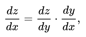
An easy analogy you can use to help you understand this better is: If a car travels twice as fast as a bicycle and the bicycle is four times as fast as a walking man, then the car travels 2 x 4 = 8 times as fast as a walking man.
This tells us that the correct thing to do here is to multiply. We are taking these intermediary rates of change and we are multiplying them together.
So if we use this now to derive dL / dc, well if that is what we want, let't look at what we have. We have dL / dd = -2.0 and dd / dc = 1.0 (1.0 because this is a plus node). So the chain rule tells us to multiply them to figure out dL / dc = -2.0 * 1.0 = -2.0. So we basically we just copy over the -2.0 value because the other one is just 1.0, so literally what a plus node does is it just routes the gradient along the graph because the plus node's local derivatives are just 1.0.
So c.grad = -2.0 and by symmetry e.grad = -2.0 as well. Filling this in and re-drawing our visualisation we get:

Now we are going to recurse our way backwards again one final time for the last two nodes and fill out their grad values and we are again going to apply the chain rule.
We have dL / de = -2.0, we have just calculated this, so we know the derivative of L with respect to e. And now we want dL / da = ?, the chain rule tells us that that is just (dL / de) * (de / da). So because we have that e = a * b, the derivative of that with respect to a is just b.
So now we know that a.grad = -2,0 * -3.0 = 6.0, by symmetry b.grad = -2.0 * 2.0 = -4.0. Let's re-draw!

That's it! That was backpropogration done manually! Literally all we did was iterate through all the nodes one by one and locally applied the chain rule. That's really what backpropogation is, just a recursive application of the chain rule backwards through the computation graph.
Let's briefly see this in action. Let's try to nudge our inputs to try to make L go up. So lets start with a.data and if we want L to go up we just need to go in the direction of the gradient. So a should increase in the direction of the gradient by some small amount (this is the step size): a.data += 0.001 + a.grad.
We also want this for all four of our leaf nodes which we usuaully have control over.
a.data += 0.001 + a.grad
b.data += 0.001 + b.grad
c.data += 0.001 + c.grad
f.data += 0.001 + f.grad
Again, if we run this, because we are nudging in the direction of the gradient we are expecting L to go up. It's current value is -8.0 so it should become less negative. Running that and printing L.data we get -7.286496. Ok nice, just as we expected.
This is basically one step of an optimisation that we'll end up running, so really these gradients give us this power, with them we know how to influence the final outcome. This is extremely useful for training neural nets.
Now lets go through and do a more complex and more useful example by backpropogating through a Neuron.
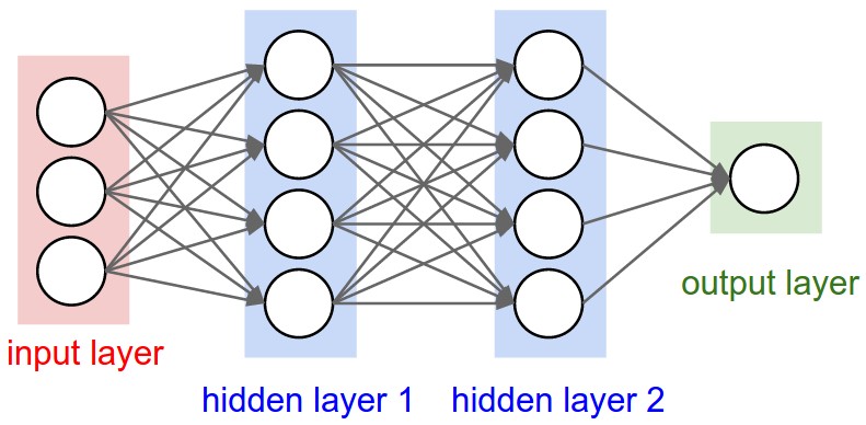
So we want to eventually build out neural networks, and in the simplest case this is a multilayer perceptron (MLP), for example this is a 2 layer neural net and its got these two hidden layers made up of neurons which are connected to each other through the layers.
Biologically neurons are very complicated devices.
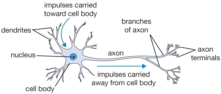
But we have very simple mathematical models of them.
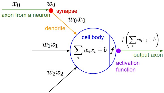
You have some input (xs) and then you have these synapses (ws) that have weights attatched to them. The synapse interacts with the input to this neuron multiplicatively so what flows to this cell body of this neuron is w * x. But there can be multiple inputs so there can be many wx's flowing into this cell body. The cell body also then has some sort of bias, so this is like the innate trigger happiness to this neuron. Essentially we are taking all the wx's adding the bias and then take it through some activation function which is usually some kind of squashing function like a sigmoid or tanh.
Here, I am going to use the tanh, lets quickly visualise this using numpy with this code:
plt.plot(np.arange(-5, 5, 0.2), np.tanh(np.arange(-5, 5, 0.2))); plt.grid()this outputs this image showcasing what a tanh function looks like:
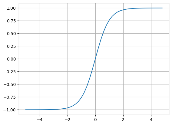
You can see that as the inputs come in get squashed on the y coordinate, so right at 0 we get exactly 0, then as you go more positive in the input then the function will only go up to 1 and same thing on the reverse side with -1. So if you pass in very positive numbers we cap them smoothly at 1 and same thing on the negative side but capping to -1.
So that is the activation function, and what comes out of the neuron is just the activation function applied to the dot product of the weights and the inputs.
So if we write one out with this code:
# inputs x1,x2
x1 = Value(2.0, label='x1')
x2 = Value(0.0, label='x2')
# weights w1,w2
w1 = Value(-3.0, label='w1')
w2 = Value(1.0, label='w2')
# bias of the neuron
b = Value(6.7, label='b')
# x1*w1 + x2*w2 + b
x1w1 = x1*w1; x1w1.label = 'x1*w1'
x2w2 = x2*w2; x2w2.label = 'x2*w2'
x1w1x2w2 = x1w1 + x2w2; x1w1x2w2.label = 'x1*w1 + x2*w2'
n = x1w1x2w2 + b; n.label = 'n'
Here we have the inputs of this neuron (x1 and x2, so its a two dimensional neuron), then you have the weights of the neuron (w1, w2, these are the synaptic strengths of each input) and finally the bias of the neuron (b). Then, according to that model above, we multiply x1 * w1 and x2 * w2 and then we need to add bias on top of it. So now n is the cell body's raw activation without the activation function for now. Now let's draw this with draw_dot(n):

Now lets's take it through an activation function, let's use the tanh function so that we can produce the output. We can add onto the end o = n.tanh(), only issue is that we haven't yet written the tanh function for our Value class. So far we have only a plus and a times, and you cannot create this hyperbolic function out of just plusses and times, you also need exponentiation.
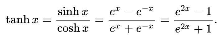
So this is the tanh formula and you can see that it also requires exponentiation as well as division, so we are not able to produce tanh yet, we are gonna go back to the Value class and implement something like it. Now we don't actually have to implement this tanh implementation using the exponents. We are actually completely free to implement functions at arbitrary points of abstraction. The only thing that matters is that we know how to differentiate through any one function.
So instead of implementing division and exponentiation lets just implement tanh directly:
def tanh(self):
    x = self.data
    t = (math.exp(2*x) - 1) / (math.exp(2*x) + 1)
    out = Value(t, (self, ), 'tanh')
    return out
Now Value should be implementing tanh and we can come back and use it in here and aso then draw the output node instead of n.
# inputs x1,x2
x1 = Value(2.0, label='x1')
x2 = Value(0.0, label='x2')
# weights w1,w2
w1 = Value(-3.0, label='w1')
w2 = Value(1.0, label='w2')
# bias of the neuron
b = Value(6.7, label='b')
# x1*w1 + x2*w2 + b
x1w1 = x1*w1; x1w1.label = 'x1*w1'
x2w2 = x2*w2; x2w2.label = 'x2*w2'
x1w1x2w2 = x1w1 + x2w2; x1w1x2w2.label = 'x1*w1 + x2*w2'
n = x1w1x2w2 + b; n.label = 'n'
o = n.tanh(); o.label = 'o'
draw_dot(o)
But remember we must know the derivative of tanh in order to backprop through it.
Let's quickly do something a little strange, lets change the bias to this number instaed 6.8813735870195432, this is because we are about to start backpropogation and using this weird number will give us nice numbers as outputs so its easier to understand essentially. So let's start filling in all the grads with backprop.
So what is the derivative of o with respect to o? This is our base case and remember this is just 1.0, so let's set that with o.grad = 1.0.

So if we have o = tanh(n), so what is the derivative of o with respect to n? Now you could go do the whole differentiation of that whole exponential expression or we could just use this:
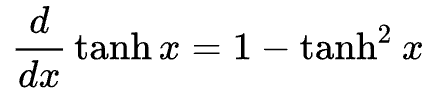
This tells us that do / dn = 1 - (tanh(n)**2) = 1 - o**2. Ok so let's use that now, we know that o.data = 0.6044 and so n.grad would just be 1 - 0.6044**2 which is gives us 0.4999999999999999... so the local derivative of this tanh operation here is conveniently 0.5 lol. We can now fill this in our graph with n.grad = 0.5 giving us this graph.

Ok now, let's continue this backprop, next we have a plus node, so we just route the grad over to the next nodes, giving us.
Continuing once again with a second plus node, we get:

Now continuing to backprop through the times nodes, first the x1 and w1 nodes. So for x1.grad = 0.5 * -3.0, for w1.grad = 0.5 * 2.0, and doing the same thing for x2 and w2 and finally visualising it all we get this graph:

Finally, we are done with this manual backpropogation, let's put an end to this suffering and automate this backward pass. But this needed to be done to make it extra clear by example how exactly backprop works, and what it's really doing behind the scenes.
Let's go back up to our Value class and let's start codifying this process. We are going to start by storing a special self._backward variable in our values which will hold a function which will essentially do that little piece of chain rule at each little node. By default this will be a function that doesn't do anything so we use:
self._backward = lambda: NoneThe reason why it initially does nothing is for the leaf node cases where there is nothing to do.
But when we are creating these out values in the other op functions we do need to set this _backward variable to something. If we start with the __add__, here we need to set the _backward to be the function that propagates this gradient. For addition our job is to take out's grad and propagate it to self's grad and other's grad.
def __add__(self, other):
    out = Value(self.data + other.data, (self, other), '+')

    def _backward():
        self.grad = 1.0 * out.grad
        other.grad = 1.0 * out.grad

    out._backward = _backward()
    return out
Let's now do multiplication.
def __mul__(self, other):
    out =  Value(self.data * other.data, (self, other), '*')

    def _backward():
        self.grad = other.data * out.grad
        other.grad = self.data * out.grad

    out._backward = _backward()
    return out
And finally for tanh too:
def tanh(self):
    x = self.data
    t = (math.exp(2*x) - 1) / (math.exp(2*x) + 1)
    out = Value(t, (self, ), 'tanh')

    def _backward():
        self.grad = (1 - t**2) * out.grad

    out._backward = _backward()
    return out
Now we dont have to do this manually anymore, if we re-initialise the data so our grad values are all 0.0 again. We now just need to call this _backward() function in the right order. As a base case we need to set o.grad to 1.0 instead of the 0.0 that it initially starts with. So now calling o._backward() gives us this:

As you can see it has automatically filled in n.grad to 0.5 as it should be. Now continuing with the rest of them:
o._backward()
n._backward()
x1w1x2w2._backward()
x1w1._backward()
x2w2._backward()
and if we check now what everything is:
Perfect, everything is filled out and is correct.
But now, we still had to manually call the _backward() methods manually so we actually have one last piece to get rid of. So let's take care of that.
Essentially what we did was we laid out this mathematical expression and we are trying to backwards through that. Now going backwards through our expression just means that we never want to call the function on any node before we have done everything after it. So this ordering of graphs can be achieved through something called a topological sort.
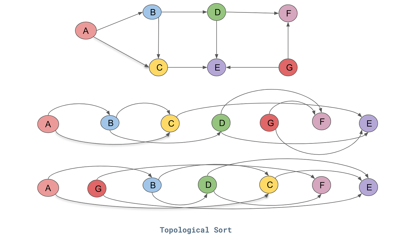
Topological sort is basically a laying out of a graph such that all the edges only go from left to right. As you can see above we start with a directed acyclic graph (DAG) and below are two different topological sorts of it where it basically lays out the nodes such that all the edges go in one direction. To implement this we use this code below:
topo = []
visited = set()
def build_topo(v):
    if v not in visited:
        visited.add(v)
        for child in v._prev:
            build_topo(child)
        topo.append(v)
build_topo(o)
topo
Basically this is what builds our topological graph, we maintain a set of visited nodes and then starting at some root node (which for us its o, that's where we want to start the topological sort). So starting at o we go through all of its children and we need to lay them out from left to right. So it starts at o, if its not visited then it marks it as visited and then it iterates through all of its children and calls the build_topo() on them and then after it has gone through all of its children it adds itself. So our node o is only going to add itself to the topo list after all of its children have been processed. So now if we inspect this list:
[Value(data=6.881373587019543),
 Value(data=2.0),
 Value(data=-3.0),
 Value(data=-6.0),
 Value(data=1.0),
 Value(data=0.0),
 Value(data=0.0),
 Value(data=-6.0),
 Value(data=0.8813735870195432),
 Value(data=0.7071067811865476)]
So now all thats left to do is to call _backward() on all of the nodes in the topological order.
So from the start now, first we start by setting o.grad = 1.0, thats the base case, then we build the topological order and then we call the _backward() function for each node in the reversed() order of topo. Codifying that we get:
o.grad = 1.0

topo = []
visited = set()
def build_topo(v):
    if v not in visited:
        visited.add(v)
        for child in v._prev:
            build_topo(child)
        topo.append(v)
build_topo(o)

for node in reversed(topo):
    node._backward()
We can quickly check if that is good by re-initialising our expression to clear the grads, then run that code and see if the grads are all filled in, which they are.
Finally, we are going to hide this functionality inside the Value class so we dont just have all that code lying around. So instead of an _backward() we are now going to define an actual backward().
def backward(self):
    topo = []
    visited = set()
    def build_topo(v):
        if v not in visited:
            visited.add(v)
            for child in v._prev:
                build_topo(child)
            topo.append(v)
    build_topo(self)

    self.grad = 1.0
    for node in reversed(topo):
        node._backward()
So now we can just call o.backward() without the underscore and there we go. And that is backpropogation!
Actually, all is not well... there is actually a bug in our code that we have not noticed because of some certain conditions that we need to think about. Here is the simplest case that shows the bug:
a = Value(3.0, label='a')
b = a + a; b.label = 'b'
b.backward()
draw_dot(b)
If we run that we see this graph:

Let's say we create a single node a and then I create a node b that is a + a and then I called backward(). In the graph it looks like there is one arrow there connecting to the plus node but actually there are 2! Looking at the forward pass it works, a + a is indeed 6.0, but the gradient there is not actually correct. You should easily be able to spot this because by doing the differentiation of that b expression with respect to a should actually be 2 (1 + 1) not 1. Essentially what is happening is we are overriding the gradient because self and other (in the add method) are both a, but our code is assigning 1 to them twice.
This issue will arise any time you use a variable more than once, since until now we haven't done this we haven't seen the issue but that doesn't mean it shouldn't get fixed!
So the solution is actually very simple, instead of re-assigning these gradient values we need to accumulate them, this is a very simple fix for us because we can simply use += instead of the = that we are currently using. Here is our Value class now fixed.
class Value:

    def __init__(self, data, _children=(), _op='', label=''):
        self.data = data
        self.grad = 0.0
        self._backward = lambda: None
        self._prev = set(_children)
        self._op = _op
        self.label = label

    def __repr__(self):
        return f"Value(data={self.data})"

    def __add__(self, other):
        out = Value(self.data + other.data, (self, other), '+')

        def _backward():
            self.grad += 1.0 * out.grad
            other.grad += 1.0 * out.grad

        out._backward = _backward
        return out

    def __mul__(self, other):
        out =  Value(self.data * other.data, (self, other), '*')

        def _backward():
            self.grad += other.data * out.grad
            other.grad += self.data * out.grad

        out._backward = _backward
        return out

    def tanh(self):
        x = self.data
        t = (math.exp(2*x) - 1) / (math.exp(2*x) + 1)
        out = Value(t, (self, ), 'tanh')

        def _backward():
            self.grad += (1 - t**2) * out.grad

        out._backward = _backward
        return out

    def backward(self):
        topo = []
        visited = set()
        def build_topo(v):
            if v not in visited:
                visited.add(v)
                for child in v._prev:
                    build_topo(child)
                topo.append(v)
        build_topo(self)

        self.grad = 1.0
        for node in reversed(topo):
            node._backward()
We can also check if its fixed by redrawing the previous graph to make sure it is now 2.

Nice!
Ok, now, going back to the tanh function. We could have broken it down into its explicit atoms, in terms of other expressions if we had the exponential function in our Value class. But we chose to develop tanh as a single function because we knew its derivative and so we could backprop through it, however let's not forget that the atomic variant using the exp functions still exists. So now let's do exactly that, to prove that it can also be done this way and also so we can implement a couple more expressions and functions into our Value class.
First let's take care of this, currently we cannot do this:
a = Value(2.0)
a + 1
Running that would give us this error:
---------------------------------------------------------------------------
AttributeError                            Traceback (most recent call last)
Cell In[111], line 2
      1 a = Value(2.0)
----> 2 a + 1

Cell In[107], line 18, in Value.__add__(self, other)
     17 def __add__(self, other):
---> 18     out = Value(self.data + other.data, (self, other), '+')
     20     def _backward():
     21         self.grad += 1.0 * out.grad

AttributeError: 'int' object has no attribute 'data'
It says int object has no attribute data, of course, because other (now being the integer 1) doesn't have a data attribute. The integer 1 is not a Value object and we only have addition for Value objects right now. So as a matter of convenience let's fix that with this line of code:
other = other if isinstance(other, Value) else Value(other)All we are doing is checking if other is an instance of Value, if it is leave it alone, otherwise I will assume its an integer or a float and we are just going to wrap it with Value.
Now if we run the code again adding 1 to a we get: Value(data=3.0). Now we need to do the exact same thing for multiply.
Ok, so now a * 2 works and we get: Value(data=4.0) but what about if we do 2 * a? Trying to do that I get this error:
---------------------------------------------------------------------------
TypeError                                 Traceback (most recent call last)
Cell In[116], line 2
      1 a = Value(2.0)
----> 2 2 * a

TypeError: unsupported operand type(s) for *: 'int' and 'Value'
This is because when I do a * 2 python is essentially doing a.__mul__(2) but if I do it the other way around it then runs this 2.__mul__(a) and the integer 2 cannot multiply a Value object and so it gets confused. So instead we need to define something called an __rmul__ that will look like this:
def __rmul__(self, other):
    return self * other
Rmul is kind of like a fallback, so if python cannot do 2 * a it will check if by any chance a knows how to multiply by 2, and that gets called into __rmul__. So all we do in that is just swapping the order of the operands.
Ok nice, what's left now is to get exponentiation and division, in order to be able to codify the tanh exponentiation formula. Let's start with the exponentiation part.
def exp(self):
    x = self.data
    out = Value(math.exp(x), (self, ), 'exp')

    def _backward():
        self.grad += out.data * out.grad

    out._backward = _backward
    return out
We are going to introduce a single function exp(), but how do we backprop through e to the x? Well, famously, the differentiation for that is simply the exact same, e to the x, which we just stored in out.data. So apply the chain rule and we have the _backward() function complete too.
And the last thing we need to do is division. I will do this in a little bit more powerful way than just division. What we would like to work is to do something like this:
a = Value(2.0)
b = Value(4.0)
a / b
which should return 0.5 but currently gives us this error:
---------------------------------------------------------------------------
TypeError                                 Traceback (most recent call last)
Cell In[117], line 3
      1 a = Value(2.0)
      2 b = Value(4.0)
----> 3 a / b

TypeError: unsupported operand type(s) for /: 'Value' and 'Value'
Now division can actually be re-shuffled like this:
a / b
a * (1/b)
a * (b**-1)
If we have a / b, that's actually the same as a multiplying by 1 over b. Which is also the same as a multiplying by b to the power of negative 1. And so what we would really need to implement is a to the power of k (a**k), of some constant k. The reason for doing it this way is simply because its more general.
So we can redefine division like this:
def __truediv__(self, other):
    return self * (other**-1)
Now we just need to define this part other**-1, so we need to implement the __pow__() function.
def __pow__(self, other):
assert isinstance(other, (int, float)), "only supporting int/float powers for now"
out = Value(self.data**other, (self, ), f'**{other}')
def _backward():
self.grad += other * (self.data**(other - 1)) * out.grad
out._backward = _backward
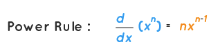
return outHere we are forcing other to essentially be either an int or a float, otherwise the math won't work for what we are trying to achieve in this specific case. And the chain rule for backproping through the power function is the derivative of the power rule.
We also need one final piece of code to be able to subtract too, of course. So we have these two:
def __neg__(self):
    return self * -1

def __sub__(self, other):
    return self + (-other)
So we have the __sub__() to be able to subtract, implemented by an addition of a negation. And to implement negation we simply multiply by negative 1.
So now a / b gives us: Value(data=0.5)! Very good!
Ok now let's go back to this graph that uses the tanh:
So now let's actually break up that tanh into the exponential equivalent.
We first start with what we currently have:
# inputs x1,x2
x1 = Value(2.0, label='x1')
x2 = Value(0.0, label='x2')
# weights w1,w2
w1 = Value(-3.0, label='w1')
w2 = Value(1.0, label='w2')
# bias of the neuron
b = Value(6.8813735870195432, label='b')
# x1*w1 + x2*w2 + b
x1w1 = x1*w1; x1w1.label = 'x1*w1'
x2w2 = x2*w2; x2w2.label = 'x2*w2'
x1w1x2w2 = x1w1 + x2w2; x1w1x2w2.label = 'x1*w1 + x2*w2'
n = x1w1x2w2 + b; n.label = 'n'
o = n.tanh(); o.label = 'o'
o.backward()
Let's change how we define o to implement this formula here:

So we need e to 2x, which is (2*n).exp(), and because we will use it twice let's create an intermediate variable e and then define o as the following:
# inputs x1,x2
x1 = Value(2.0, label='x1')
x2 = Value(0.0, label='x2')
# weights w1,w2
w1 = Value(-3.0, label='w1')
w2 = Value(1.0, label='w2')
# bias of the neuron
b = Value(6.8813735870195432, label='b')
# x1*w1 + x2*w2 + b
x1w1 = x1*w1; x1w1.label = 'x1*w1'
x2w2 = x2*w2; x2w2.label = 'x2*w2'
x1w1x2w2 = x1w1 + x2w2; x1w1x2w2.label = 'x1*w1 + x2*w2'
n = x1w1x2w2 + b; n.label = 'n'
# -------
e = (2*n).exp(); e.label = 'e'
o = (e - 1) / (e + 1); o.label = 'o'
# -------
o.backward()
Now before running this what do we expect, well all we've done is break down that tanh into a mathematically equivalent expression, so our graph might get a little longer but we should see the exact same data value for o as well as the same greadients on the rest of the nodes which would mean that our backward pass also works correctly. Let's verify.

Perfect! So this tells us that the level at which we implement operations in is totally up to us! We can implement backward passes for tiny individual operations like a plus or a minus, or we can implement them for something like a tanh function, so like composite operations.
Alright, so now let's have a look at how we can do the exact same thing but instead using a modern deep neural net library like PyTorch for example.
PyTorch is something you would of course use in production.
So this is what it would look like:
import torch

x1 = torch.tensor([2.0]).double()                ; x1.requires_grad = True
x2 = torch.tensor([0.0]).double()                ; x2.requires_grad = True
w1 = torch.tensor([-3.0]).double()               ; w1.requires_grad = True
w2 = torch.tensor([1.0]).double()                ; w2.requires_grad = True
b = torch.tensor([6.8813735870195432]).double()  ; b.requires_grad = True

n = x1*w1 + x2*w2 + b
o = torch.tanh(n)

print(o.data.item())
o.backward()

print('---')
print('x2', x2.grad.item())
print('w2', w2.grad.item())
print('x1', x1.grad.item())
print('w1', w1.grad.item())
So we first import pytorch, then we define our value objects like we did previously. Something to keep in mind is that zdravkograd is a scalar valued engine, so we only have scalar values like 2.0, but in PyTorch everything is based around tensors which are just n dimensional arrays of scalars. So thats why things get a little bit more complicated here with this type of code tensor([2.0]) because we just need a single element tensor, usually they will be larger and more complex. After that we are also casting it to be a double, this is because by default python uses double precision for its floating point numbers so we would like everything to be identical, because by default tensors use a single precision float (float32, whereas we need float64).
Another thing that we would have to do is because by default PyTorch is treating these as leaf nodes, which don't have gradients, so we need to explicitly say that all of these nodes require gradients with this code: x1.requires_grad = True. PyTorch sets these to False by default for efficiency reasons.
So once we have defined our nodes we can now perform arithmetic and also use the torch.tanh(). And just like in zdravkograd its got a data and a grad attribute, only difference is we also need to call .item() this essentially strips out the tensor part and just leaves you with the number. So if we run this we see:
0.7071066904050358
---
x2 0.5000001283844369
w2 0.0
x1 -1.5000003851533106
w1 1.0000002567688737
Which are the same values that we had with zdravkograd. So basically PyTorch can do what we did in zdravkograd as a special case when your tensors are all single element tensors. The big deal with PyTorch is everything is significantly more efficient because we are working with these tensor objects and we can do lots of operations on them in parallel on all of these tensors.
Ok, so now that we have some machinery to build out some pretty complicated mathematical expressions we can also start building out neural nets. Again keep in mind that neural nets are just a specific class of mathematical expressions.
So we are going to start building out a neural net piece by piece and eventually build out a 2 layer MLP. Let's start with a single individual Neuron.
class Neuron:
    def __init__(self, nin):
        self.w = [Value(random.uniform(-1,1)) for _ in range(nin)]
        self.b = Value(random.uniform(-1,1))
So the constructor will take number of inputs (nin), which is how many inputs come into a neuron and then its going to create a weight (w) that is some random number between negative 1 and 1 for every one of those inputs, and a bias (b) that controls the overall trigger happiness of this neuron. And then we will implement a __call__() function.
If you don't know what that function does let me show you, let's do this for now:
def __call__(self, x):
    return 0.0
The way this works now is we can do this:
x = [2.0, 3.0]
n = Neuron(2)
n(x)
Let's create some x which has two numbers in an array, then we initialise a neuron that is 2 dimensional, because we have two numbers. Then we can feed those two numbers into that neuron using n(x), and so when you use this notation n(x) python uses the __call__() method.
Ok currently though call just returns 0.0 and we need it to do w * x + b, the forward pass.
def __call__(self, x):
    act = sum((xi*wi for xi,wi in zip(x, self.w)), self.b)
    out = act.tanh()
    return out
So what we do is we multiply all of the elements of w with all of the elements of x, pairwise. So the first thing we are going to do is we are going to zip up self.w and x. In python zip() essentially takes two iterators and it creates a new iterator that iterates over the tuples of their corresponding entries. And now we multiply wi times xi and then sum all of that together to come up with an activation, and also self.b on top. So that's the raw activation and then of course we need to pass that through a squashing function (will use tanh for this for simplicity).
So now running this:
x = [2.0, 3.0]
n = Neuron(2)
n(x)
And that will give us some outputs like these:
Value(data=0.9321534794856714)Value(data=0.2873141110548085)Value(data=-0.7198429286366963)And we get a different output from the neuron each time because we are initialising different weights and biases.
Next up we are going to define a Layer of Neurons. So here we have a schematic for an MLP.
Here you can see that each layer has a number of neurons and they are not connected to each other but all of them are fully connected to the input. So all a layer of neurons is, is a set of neurons all evaluated independently.
class Layer:

    def __init__(self, nin, nout):
        self.neurons = [Neuron(nin) for _ in range(nout)]

    def __call__(self, x):
        outs = [n(x) for n in self.neurons]
        return outs
The Layer class here is literally just a list of neurons, and then how many neurons do we have in it is just the nout variable (number of outputs). And so we just initialise completely independent Neurons with this given dimensionality. And when we call a Layer we just independently evaluate them.
And now we can create a Layer of neurons like this:
x = [2.0, 3.0]
n = Layer(2, 3)
n(x)
And calling the layer would independently evaluate them and give us something like this:
[Value(data=-0.9557290239408349),
 Value(data=0.9688743763488269),
 Value(data=0.2821627732604002)]
Okay and finally, let's complete this picture and define an MLP, and as you can see from the simple example above those layers just feed into each other sequentially.
class MLP:

    def __init__(self, nin, nouts):
        sz = [nin] + nouts
        self.layers = [Layer(sz[i], sz[i+1]) for i in range(len(nouts))]

    def __call__(self, x):
        for layer in self.layers:
            x = layer(x)
        return x
So an MLP is very similar, we are taking the number of inputs, same as before, but now instead of taking a single nout, which is the number of neurons in a single layer, we are going to take a list of nouts and this listifies the sizes of all the layers that we want in our MLP.
So in the __init__() we just put them all together and then iterate over consecutive pairs of these sizes and then create Layer objects for them. And then in the __call__() function we are just calling them sequentially. So that's an MLP really. And let's actually re-inplement this picture:
So we want 3 input neurons, then two layers of 4 and then an output.
x = [2.0, 3.0, -1.0]
n = MLP(3, [4, 4, 1])
n(x)
So we want three inputs, so make sure x has three inputs, then we initialise the MLP with three inputs, two layers of 4 and then a single output, and then calling it we get the forward pass of the MLP:
[Value(data=0.371457832931364)]To make this a little bit nicer, see how we get this output in a list, becaue Layer always returns a list, so for convenience let's do this:
return outs[0] if len(outs) == 1 else outsAnd this allows us to get a single Value out at the last layer if it only has a single neuron, like this:
Value(data=0.863842062086533)Another thing we can do is also draw dot this n(x) and as you might imagine these expressions are now getting quite huge:

So of course you would never go and differentiate thruogh all of this but with zdravkograd we will be able to backpropogate all the way through this, and backprop into these weights of all these neurons, so let's see how that works.
First, let's create a simple example dataset here:
xs = [
    [2.0, 3.0, -1],
    [3.0, -1.0, 0.5],
    [0.5, 1.0, 1.0],
    [1.0, 1.0, -1.0]
]
ys = [1.0, -1.0, -1.0, 1.0]
So this dataset has 4 examples (xs), and so we have 4 possible inputs into the neural net. We also have 4 desired targets (ys), so we would like the neural net to output 1.0 when its fed the first example and so on. So it's a very simple binary classifier neural net that we would like here.
Now let's see what the neural net currently thinks about these 4 examples using this:
ypred = [n(x) for x in xs]
ypred
We just get their predictions, all we are doing is calling n(x) for x in xs and then we can print:
[Value(data=0.863842062086533),
 Value(data=0.39251845122664425),
 Value(data=0.8794808525523493),
 Value(data=0.8461914035578225)]
So these are the outputs of the neural net, so these are the outputs of the neural net for those 4 examples. So the first one is 0.863842062086533 but we would like it to be 1.0 so we should push this one higher. The second one says 0.39251845122664425 and we would like that one to be -1.0 so that should go down, and so on.
So now how do we tune the weights of the neural net to better predict the desired targets? The trick used in deep learning to achieve this is to calculate a single number that somehow measures the total performance of our neural net, and we call this single number the loss. Right now we have the intuitive sense that it's not performing very well because we are not very close to our desired outputs (ys), so the loss will be high, we want to minimise the loss.
So in this particular case we are going to implement a mean squared error loss.
for ygt, yout in zip(ys, ypred)What this is doing is pairing the ground truths with the predictions, and that zip iterates over tuples of them.
[(yout - ygt)**2 for ygt, yout in zip(ys, ypred)]And for each y ground truth and y output we are going to subtract them and square them. So let's first see what these losses are (the individual loss components):
[Value(data=0.018538984056847528),
 Value(data=1.9391076370066518),
 Value(data=3.532448275110905),
 Value(data=0.02365708433951261)]
Basically, for each one of the four, we are taking the prediction and the ground truth, we are subtracting them and squaring them. Instead of squaring we could also take the absolute value, we just need to discard the sign. And so the expression is arranged so that you only get 0 if y out is equal to y ground truth, when those two are equal, so your prediction is exactly the target we will get 0. The more off our predictions are the greater the loss will be. We don't want high loss we want low loss.
And so the final loss will simply be the sum of all of those numbers:
loss = sum((yout - ygt)**2 for ygt, yout in zip(ys, ypred))
loss
Which gives us:
Value(data=5.513751980513917)So now we need to minimise the loss because if loss is low then every one of our predictions is equal to its target.
Now, if we do loss.backward(), something magical may happen...
We can take a look at this: n.layers[0].neurons[0].w[0].grad which now gives us -0.15455925201254145, so it now has a grad, thanks to the backward pass. So we see here that this weight here of this particular neuron in this particular layer is negative, this tells us that it's influence on the loss is also negative. So slightly increasing this weight would make the loss go down. And we have this information for every one of our neurons and all of their params.
It's also worth looking at the draw_dot() of the loss, remember previously we looked at the graph of a single neuron's forward pass and that was already a large expression, but what is this expression? We actually forwarded every one of those 4 examples and then we have the loss on top of them with the mean squared error and so what we get is a super duper massive graph.

You can see also that all of these nodes have their grads too, even the input data, but the grads for the input data aren't very useful to us, this is because they are fixed and cannot be changed. However, some of these gradients will be for the neural network parameters, the w's and the b's and those of course we want to change.
Ok so now we want some convenience code that will essentially gather up all of the parameters of the neural net so we can operate on them simultaneously, and every one of them we will nudge a tiny amount based on the gradient information. So let's collect the parameters of the neural net now all in one array.
def parameters(self):
    return self.w + [self.b]
We put this in our Neuron class, we return self.w which is a list, concatenated with a list of self.b. List plus list equals list, simple.
def parameters(self):
    return [p for neuron in self.neurons for p in neuron.parameters()]
This goes in our Layer class and here we just use a single list comprehension.
def parameters(self):
    return [p for layer in self.layers for p in layer.parameters()]
And finally in our MLP class, the same thing pretty much as the previous one.
Ok now we are going to need to re-initialise our network so we will lose the values we were just looking at but thats fine. So now if we do n.parameters() we get this:
[Value(data=-0.8015031074224241),
 Value(data=-0.9169580898178005),
 Value(data=0.8556360302178518),
 Value(data=-0.40745808569150066),
 Value(data=0.35499781299863375),
 Value(data=0.40324357016872847),
 Value(data=-0.08197521469981339),
 Value(data=0.15258478301306333),
 Value(data=0.2620667957020506),
 Value(data=0.20325364452614703),
 Value(data=0.16693492897014472),
 Value(data=-0.2825010088926958),
 Value(data=0.9075135652459132),
 Value(data=-0.6727934237259026),
 Value(data=0.8130353342221799),
 Value(data=-0.9633407928660425),
 Value(data=-0.0511356434988357),
 Value(data=-0.019318335169764334),
 Value(data=0.2768318434993102),
 Value(data=0.4467459999768564),
 Value(data=-0.5680594358215434),
 Value(data=-0.8300702788390601),
 Value(data=0.11923328682833767),
 Value(data=0.9134430140647103),
 Value(data=0.8020264888226167),
 Value(data=-0.9987514138253692),
 Value(data=-0.8985516792314467),
 Value(data=0.6217507843036687),
 Value(data=0.26861330170360675),
 Value(data=-0.620341103739469),
 Value(data=-0.617633298138331),
 Value(data=-0.8790622221055819),
 Value(data=0.8917832461492952),
 Value(data=-0.14110333866554758),
 Value(data=0.7802349008255729),
 Value(data=-0.34409641719983153),
 Value(data=-0.13489395330055864),
 Value(data=-0.5266494915790159),
 Value(data=0.9323603822462916),
 Value(data=0.3478018151186828),
 Value(data=-0.3671053115302143)]
So these are all the weights and biases of the entire neural net, so in total (len(n.parameters()) = 41), this MLP has 41 parameters.
Ok so we see now that this neuron's gradient n.layers[0].neurons[0].w[0].grad which is -1.2981844955870419 is slightly negative. We can also look at its data with n.layers[0].neurons[0].w[0].data which is -0.9226360174816963.
So what we want to do now is iterate for every parameter in our n.parameters(), so for all the 41 parameters in this neural net, we want to change p.data slightly according to the gradient information. So this will be a tiny update in our gradient descent scheme. In gradient descent we are thinking of the gradient as a vector pointing in the direction of increasing loss.
for p in n.parameters():
    p.data -= 0.01 * p.grad
So if we run this, and nudge all the params a tiny amount, then we can see that this data n.layers[0].neurons[0].w[0].data has now changed to this number -0.9096541725258259, it changed slightly. So now its a little bit greater of a value, and that's a good thing because slightly increasing this neuron will make the loss go down, according to its gradient.
So now because we have changed all these values we can expect that the loss which used to be Value(data=4.536247811077203) should have gone down a bit, it's now Value(data=3.6754712071009727). Good and remember, low loss means that our predictions are now closer to the targets!
So now what we have to do is we have to iterate this process. Keep in mind also that if you try to go too fast and try to make too big of a step you may actually overstep the local minimum of the gradient. This can destabalise training and make the loss blow up even.
Now let's make this a tiny bit more respectable and implement an actual training loop. This is the data definition:
xs = [
    [2.0, 3.0, -1],
    [3.0, -1.0, 0.5],
    [0.5, 1.0, 1.0],
    [1.0, 1.0, -1.0]
]
ys = [1.0, -1.0, -1.0, 1.0]
Then, first we do a forward pass, then we do a backward pass and finally we update the params.
for k in range(20):
    # forward pass
    ypred = [n(x) for x in xs]
    loss = sum((yout - ygt)**2 for ygt, yout in zip(ys, ypred))
    # backward pass
    loss.backward()

    # update
    for p in n.parameters():
        p.data -= 0.05 * p.grad

    print(k, loss.data)
And if we run this we get this:
0 1.529599185105458
1 2.3051303835639994
2 0.1591446736518378
3 0.10273687114381344
4 0.13397239276922573
5 0.18270233530130778
6 0.046404137513044605
7 0.005438687988357785
8 0.005108786902330618
9 0.028666411491592398
10 0.14781510657782143
11 0.05577413010013488
12 0.0012665326175115665
13 1.2506186958400938e-05
14 3.8045143707629016e-07
15 3.6794105378802586e-08
16 5.138244152180156e-09
17 8.25893563724724e-10
18 1.4696623456863828e-10
19 2.8584294814650368e-11
Nice, we have converged, we got to a loss that is very low! So now let's inspect ypred and see if its close to our ys:
[Value(data=0.9999965916090436),
 Value(data=-0.9999993082504521),
 Value(data=-0.9999994833141905),
 Value(data=0.9999959723847949)]
Yes! It's super duper close!
However, there is an issue, and its a very common issue that even experts can forget and fall into. We forgot to zero grad! What is that? It's quite subtle but essentially, all of these weights have a .data() and a .grad(). The .grad() starts at 0, then we do a backward pass which fills in the gradients, then we do an update on the data using those grads, and after that we don't flush the grad, it stays there. So when we do the second forward pass, and we do backward again, remember that all the backward operations do a += on the grad, and so these gradients just add up and up and up and never get reset!
So here's how we zero grad:
for k in range(20):
    # forward pass
    ypred = [n(x) for x in xs]
    loss = sum((yout - ygt)**2 for ygt, yout in zip(ys, ypred))

    # zero gradients
    for p in n.parameters():
        p.grad = 0.0

    # backward pass
    loss.backward()

    # update
    for p in n.parameters():
        p.data -= 0.05 * p.grad

    print(k, loss.data)
We need to iterate over all the aprams and we need to make sure that the grad's are set to zero, just like it does in the constructor. So now let's reset the neural net, the data (which is the same), and if we inspect the data now:
0 10.541041025299343
1 5.591497943422341
2 2.21822735107375
3 1.2588682967425895
4 0.740132402735687
5 0.4753853358167178
6 0.3336289959698347
7 0.25042323641867265
8 0.1973719936929933
9 0.16125658883237295
10 0.13538422045670398
11 0.11609146635371728
12 0.10123628671954024
13 0.08949563146834486
14 0.08001416478133207
15 0.07221734805665654
16 0.06570653471964506
17 0.06019733451868971
18 0.0554819399134662
19 0.05140529391281888
I notice that we get a much more gradual descent, we still end up with pretty good results:
[Value(data=0.9171422487757221),
 Value(data=-0.9470136206082874),
 Value(data=-0.8524257310012262),
 Value(data=0.8587407854215888)]
Ok so why did it actually end up working with that bug in the gradient descent code?
That is because this is actually a very very simple problem that we are trying to solve with this neural net, it's very easy for this neural net to fit this data. So that grads ended up accumulating and effectively gave us a massive step size which made us converge extremely fast. So now we have to do more steps. We can also increase the step from 0.05 to 0.1 and also increase the number of steps from 20 to 100 let's say. Let's try that and see our results:
for k in range(100):
    # forward pass
    ypred = [n(x) for x in xs]
    loss = sum((yout - ygt)**2 for ygt, yout in zip(ys, ypred))

    # zero gradients
    for p in n.parameters():
        p.grad = 0.0

    # backward pass
    loss.backward()

    # update
    for p in n.parameters():
        p.data -= 0.1 * p.grad

    print(k, loss.data)
0 7.723709992198133
1 7.543538936295437
2 7.013975992374648
3 4.667171772402771
4 1.925944726113833
5 2.430507827200392
6 0.04090262825707465
7 0.03636529903661968
8 0.03272692803583811
9 0.029743371812566026
10 0.027252034637224525
11 0.02514027010150074
12 0.023327484457525353
13 0.02175445082662786
14 0.020376646166501963
15 0.01915994293001845
16 0.01807773582234216
17 0.01710897386162344
18 0.01623678079828426
19 0.015447467992139776
20 0.014729815152644557
21 0.014074537672604758
22 0.01347388634005692
23 0.012921342524542993
24 0.012411383256733757
...
96 0.003133501847820981
97 0.003100472618394274
98 0.003068116818594674
99 0.003036414227238456And our predictions with this now are:
[Value(data=0.9848083610425493),
 Value(data=-0.9690138349567345),
 Value(data=-0.9750907304087836),
 Value(data=0.9649997971810371)]
Pretty good! So I have noticed that working with neural nets can be sometimes quite tricky because there might be lots of bugs in the code and your network might actually work, just like ours worked, but chances are that if we had a more complex problem this might not have worked, we only really got away with it because the problem was very simple.
So now let me bring everything together and summarise what I have learned.
What are neural nets?
Neural nets are these mathematical expressions, fairly simple mathematical expressions in the case of MLP's, that take input as the data as well as the weights and biases of the NN. So a mathematical expression for the forward pass followed by a loss function, and the loss function tries to measure the accuracy of the predictions. And usually your loss will be low when your predictions are matching your targets, so the network is behaving well. So we manipulate the loss function so that when the loss is low, the network is doing what you want it to do on your problem. And then we backward the loss, use backpropogation to get the gradient and then we know how to tune the parameters to decrease the loss locally. But then we have to iterate that process many times in what's called a gradient descent. So we simply follow the gradient information and that minimises the loss. And that's pretty much it.
This is a very tiny network with 41 parameters but you can build significantly more complicated neural nets with billions at this point almost trillions of parameters and it's a massive blob of neural tissue, simulated neural tissue roughly speaking, and you can make it do extremely complex problems and these neurons then have all kinds of very fascinating emergent properties when you try to make them do significantly hard problems. As in the case of GPT for example, we have massive amounts of text from the internet and we're trying to get a neural net to predict to take like a few words and try to predict the next word in a sequence that's the learning problem. It turns out that when you train this on all of internet the neural net actually has like really remarkable emergent properties but that neural net would have hundreds of billions of parameters, but it works on fundamentally the exact same principles. The neural net of course will be a bit more complex but otherwise the value in the gradient is there and would be identical and the gradient descent would be there and would be basically identical but people usually use slightly different updates, this is a very simple stochastic gradient descent update and the loss function would not be mean squared error they would be using something called the cross-entropy loss for predicting the next token so there's a few more details but fundamentally the neural network setup and neural network training is identical.
Now it's time to move away from this simple backprop and actually tackle a real machine learning problem: binary classification on a non-linear dataset.
We first start off by having our usual imports at the top!
import random
import numpy as np
import matplotlib.pyplot as plt
%matplotlib inline
So in our previous problem we had this code:
xs = [
    [2.0, 3.0, -1],
    [3.0, -1.0, 0.5],
    [0.5, 1.0, 1.0],
    [1.0, 1.0, -1.0]
]
ys = [1.0, -1.0, -1.0, 1.0]
There were 4 data points but deep learning needs lots of data, we don't want to type out 100 or 1000 points manually. So we use this code here:
from sklearn.datasets import make_moons
X, y = make_moons(n_samples=100, noise=0.1)
y = y*2 - 1
What is sklearn? Scikit-learn is the industry standard machine learning library for python, It contains massive amounts of algorithms (like Random Forests, K-Means) and crucially datasets! It allows me to generate synthetic data to test my neural net.
What is make_moons? It is a specific function inside sklearn. It generates a dataset that looks like two crescent moons interlocking. Something like this:
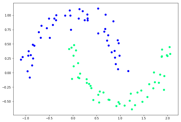
Why Moons? This is a specific stress test for classifiers. If you have two blobs of data far apart, you can draw a straight line between them. A "Linear Classifier" (like a single neuron) can solve that. But Moons dataset is non-linear, you cannot seperate the two moons with a single straight line. You need a curvy line. This will prove that our neural network is learning complexity.
What about y = y*2 - 1? Make moons returns labels (y) that are 0 (for moon A) and 1 (for moon B). Our zdravkograd logic (and the SVM we will use later) prefers -1 and +1.
So if y = 0 then 0*2 - 1 = -1, and if y = 1 then 1*2 - 1 = 1. This is just a rescaling trick to get the targets into the format that our Loss function will like.
What is ReLU? In the context of zdravkograd we used tanh, this is a smooth S curve that squashes inputs between -1 and 1. ReLU stands for Rectified Linear Unit, sounds fancy but it's actually the most simple thing in the entire world of deep learning.
f(x) = max(0, x), if the input is negative (e.g. -5), the output is 0. If the input is positive (e.g. 5) then the output is 5.
We have to switch to this from the tanh for simplicity and speed. Computing tanh requires exponentials and division. Whereas computing ReLU is just if x > 0, it is incredibly fast for the computer.
The Vanishing Gradient Problem: Tanh is flat at ends, if our neuron output is a high number (like 100) then the slope of tanh is basically 0. The gradient vanishes and the neuron stops learning. ReLU is linear for all positive numbers, the slope is always 1 so the gradient flows through perfectly.
This is the relu function that we need to add to our engine:
 def relu(self):
    out = Value(0 if self.data < 0 else self.data, (self,), 'ReLU')

    def _backward():
        self.grad += (out.data > 0) * out.grad
    out._backward = _backward

    return out
We do this the same way we added the tanh and for reference this is what the graph of relu function looks like:

In the code we first do the forward pass, out = Value(0 if self.data < 0 else self.data, (self,), 'ReLU'), it's super simple, we just codify this formula: f(x) = max(0, x). For the backward pass we need to know: what does the slope look like? Well for the positive side the line is just y = x`, if you increase x by 1, y increases by 1, so the slope is 1. And for the left side there is no slope, so the gradient is 0. The derivative is a simple switch really.
A new class needs to be added to our Neuron setup, you can see the new implementation in nn.py. We first need a new Module class:
class Module:

    def zero_grad(self):
        for p in self.parameters():
            p.grad = 0

    def parameters(self):
        return []
This is the parent class, notice that all the others now inherit this class (e.g. class Neuron(Module):), we do this so we keep it DRY (Don't Repeat Yourself). If we wanted to add a function like zero_grad, we would have to copy paste it into Neuron and the other classes, now we write it once and everyone gets it for free. zero_grad is now also its own function for code simplicity.
The updated Neuron class:
class Neuron(Module):

    def __init__(self, nin, nonlin=True):
        self.w = [Value(random.uniform(-1,1)) for _ in range(nin)]
        self.b = Value(0)
        self.nonlin = nonlin

    def __call__(self, x):
        act = sum((wi*xi for wi,xi in zip(self.w, x)), self.b)
        return act.relu() if self.nonlin else act
The bias is now 0, this is standard practice, we want our neurons to be "neutral" at the start, we only want it to fire if the weights find a pattern in the input and random bias adds unnecessary noise at the beginning.
The nonlin flag has also been added, if the output goes through the act.relu() this is set to true, but if the output is just act then it's set to false, because that would keep it a Linear Neuron.
The updated Layer class:
class Layer(Module):

    def __init__(self, nin, nout, **kwargs):
        self.neurons = [Neuron(nin, **kwargs) for _ in range(nout)]
We need this new kwargs special attribute which stands for keyword arguments, since Layer creates Neurons, we need a way to pass down that nonlin flag through the layer down to the neuron. So with it, if i call Layer(2, 3, nonlin=False), python packs nonlin=False into kwargs. Then the Neuron(nun, **kwargs) unpacks it, effectively calling Neuron(nin, nonlin=False).
And finally the updated __repr__ method, this is purely for printing but this updated one:
def __repr__(self):
    return f"{'ReLU' if self.nonlin else 'Linear'}Neuron({len(self.w)})"
Allows us to debug the architecture just by printing the object. This has no effect on the math.
Now what is SVM and Hinge Loss? SVM stands for Support Vector Machine, it is a classic machine learning algorithm (pre deep learning). The goal of an SVM is to find the "widest street" (margin) that separates two classes of data.
In zdravkograd I used mean squared error (y_pred - y_target)**2, this will try to make the prediction exactly match the target number. If the target is 1 and the prediction is 1.5, MSE tells it to go back to 1.
SVM (Hinge Loss) doesn't care about "exactness", it cares about correctness and confidence.
This is the formula: L = max(0, 1 - (y_target * y_pred)).
If target is 1 and prediction is 1.5, hinge loss says: "Great! You are correct (positive) and confident (greater than 1). Loss is 0, carry on."
The code:
losses = [(1 + -yi*scorei).relu() ...]This is the zdravkograd implementation of hinge loss, yi is for -1 or 1, scorei is the model output. If yi and scorei have the same sign (correct prediction) then yi*scorei is positive. We want yi*scorei to be greater than 1. So (1 - (yi*scorei)) measures how much we failed to beat the margin of 1. .relu() ensures that if we did beat the margin (negative result inside the brackets) the loss is clamped at 0.
Regularisation: L2 Penalty.
alpha = 1e-4
reg_loss = alpha * sum((p*p for p in model.parameters()))
This is called L2 Regularisation (or Weight Decay). Imagine the neural net finds a solution where one weight is 10,000 and another is -9,999. They almost cancel out but the math gets unstable. The decision boundary becomes incredibly jagged and weird to fit specific noisy points.
So what we do is we add a term to the loss function "The sum of all the weights squared.".
The optimiser (backprop) now has two goals:
- Make the classification correct (data loss)
- Make all the weights as small as possible (reg loss)
alpha (1e-4) is the strength, it says to the model that prediction accuracy is 10,000x more important than small weights, but please try to keep the weights small if you can."
This results in a smoother decision boundary.
In the problem we previously solved using zdravkograd we passed the entire dataset (all 4 points) into the forward pass every single step. This is fine for 4 points, but what if you had 1,000,000 images? You cannot fit 1 million images into memory all at once.
Batching means we randomly select a small chunk (e.g. 32 items) of data:
- Calculate loss on those 32
- Update the weights
- Pick a new 32
- Repeat
This is called Stochastic Gradient Descent (SGD). It is noisy (because you only see a few examples at a time), but it is much faster and allows us to train on massive datasets. In this specific demo, batch size defaults to None, so we are actually using the whole dataset, but the code is setup to handle batches if we wanted to.
Ok now that we have our library zdravkograd and our dataset understanding, let's build the actaul training script and break it down step by step.
import random
import numpy as np
import matplotlib.pyplot as plt
%matplotlib inline
Of course we first start with our imports.
from zdravkograd.engine import Value
from zdravkograd.nn import Neuron, Layer, MLP
We will also bring in Value, Neuron, Layer and MLP from the library we just built.
np.random.seed(1337)
random.seed(1337)
Now these two lines, in machine learning we use random numbers constantly, to initialise weights, to shuffle data, etc. If we just let the computer pick random numbers then every time we run this notebook, we would get slightly different results. That makes debugging a nightmare. By "seeding" the random number generator, we are telling the computer to be random but be random in the exact same way every time. This ensures that if you run the code, you will get the exact same results that I do.
Next up, the data.
# make up a dataset

from sklearn.datasets import make_moons, make_blobs
X, y = make_moons(n_samples=100, noise=0.1)

y = y*2 - 1 # make y be -1 or 1
# visualize in 2D
plt.figure(figsize=(5,5))
plt.scatter(X[:,0], X[:,1], c=y, s=20, cmap='jet')
Here we generate the "Moons" dataset, as mentioned before, we shift y to be -1 or 1 to play nice with our SVM loss. Finally we plot it to see what we are dealing with.
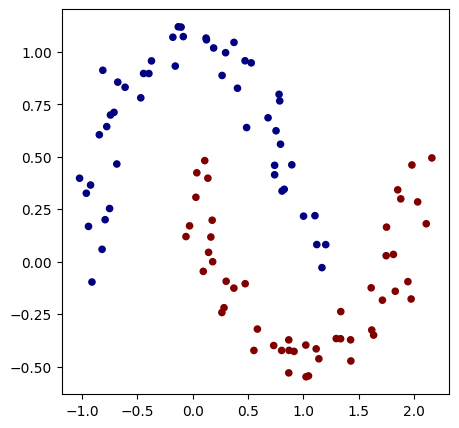
As you can see, this is the binary classification problem. We have red dots (class -1) and blue dots (class +1). The goal of the neural net is to draw a boundary that separates them. Because they are swirling into each other, a straight line won't cut it, we need a curve.
Now let's initialise our model.
# initialise a model
model = MLP(2, [16, 16, 1]) # 2-layer neural network
print(model)
print("number of parameters", len(model.parameters()))
Here we instantiate the brain. MLP(2, [16, 16, 1]) means:
- Input: 2, because our data points have two coordinates (x, y)
- Hidden Layers: [16, 16], we have two layers of processing, each with 16 neurons. This is the "capacity" of the network
- Output: 1, the network outputs a single scalar score
MLP of [Layer of [ReLUNeuron(2), ReLUNeuron(2), ReLUNeuron(2), ReLUNeuron(2), ReLUNeuron(2), ReLUNeuron(2), ReLUNeuron(2), ReLUNeuron(2), ReLUNeuron(2), ReLUNeuron(2), ReLUNeuron(2), ReLUNeuron(2), ReLUNeuron(2), ReLUNeuron(2), ReLUNeuron(2), ReLUNeuron(2)], Layer of [ReLUNeuron(16), ReLUNeuron(16), ReLUNeuron(16), ReLUNeuron(16), ReLUNeuron(16), ReLUNeuron(16), ReLUNeuron(16), ReLUNeuron(16), ReLUNeuron(16), ReLUNeuron(16), ReLUNeuron(16), ReLUNeuron(16), ReLUNeuron(16), ReLUNeuron(16), ReLUNeuron(16), ReLUNeuron(16)], Layer of [LinearNeuron(16)]]
number of parameters 337
This output tells us that we have 337 parameters. That means there are 337 Value objects (weights and biases) inside this object that act as knobs we can turn to change the predictions.
Next up, the loss function.
# loss function
def loss(batch_size=None):

    # inline DataLoader :)
    if batch_size is None:
        Xb, yb = X, y
    else:
        ri = np.random.permutation(X.shape[0])[:batch_size]
        Xb, yb = X[ri], y[ri]
    inputs = [list(map(Value, xrow)) for xrow in Xb]

    # forward the model to get scores
    scores = list(map(model, inputs))

    # svm "max-margin" loss
    losses = [(1 + -yi*scorei).relu() for yi, scorei in zip(yb, scores)]
    data_loss = sum(losses) * (1.0 / len(losses))
    # L2 regularization
    alpha = 1e-4
    reg_loss = alpha * sum((p*p for p in model.parameters()))
    total_loss = data_loss + reg_loss

    # also get accuracy
    accuracy = [(yi > 0) == (scorei.data > 0) for yi, scorei in zip(yb, scores)]
    return total_loss, sum(accuracy) / len(accuracy)

total_loss, acc = loss()
print(total_loss, acc)
This is the most dense block of code but it is the heart of the operation.
# loss function
def loss(batch_size=None):

    # inline DataLoader :)
    if batch_size is None:
        Xb, yb = X, y
    else:
        ri = np.random.permutation(X.shape[0])[:batch_size]
        Xb, yb = X[ri], y[ri]
First we handle the data loading, if batch_size is None, we use the whole dataset. If it set like 32, we randomly shuffle the data and pick a small batch. This effectively implements SGD.
inputs = [list(map(Value, xrow)) for xrow in Xb]This line is the bridge. Xb is a numpy array of numbers. Our engine doesn't know what numpy is. So we iterate through the numpy array and wrap every single number into a Value object. Now our data is part of the computational graph.
    # forward the model to get scores
    scores = list(map(model, inputs))

    # svm "max-margin" loss
    losses = [(1 + -yi*scorei).relu() for yi, scorei in zip(yb, scores)]
    data_loss = sum(losses) * (1.0 / len(losses))
We perform the forward pass (model(inputs)) and then calculate the hinge loss. We want yi * scorei to be > 1. If it't not we incur a penalty (loss). We average this loss across the batch.
# L2 regularization
    alpha = 1e-4
    reg_loss = alpha * sum((p*p for p in model.parameters()))
    total_loss = data_loss + reg_loss
Here is the regularisation I mentioned earlier. We square every single one of those 337 parameters and sum them up. We multiply by a tiny number alpha (0.0001). This adds a small pressure to the loss function that pulls all the weights towards zero. This keeps the model simple and prevents overfitting.
# also get accuracy
    accuracy = [(yi > 0) == (scorei.data > 0) for yi, scorei in zip(yb, scores)]
    return total_loss, sum(accuracy) / len(accuracy)
Finally we calculate the accuracy just for our own eyes (is the sign of the prediction matching the sign of the label?) and return the total loss.
Next up is the optimisation loop:
# optimization
for k in range(100):

    # forward
    total_loss, acc = loss()

    # backward
    model.zero_grad()
    total_loss.backward()

    # update (sgd)
    learning_rate = 1.0 - 0.9*k/100
    for p in model.parameters():
        p.data -= learning_rate * p.grad

    if k % 1 == 0:
        print(f"step {k} loss {total_loss.data}, accuracy {acc*100}%")
We run the loop 100 times:
- Forward: Compute the loss.
- Zero Grad: Reset the gradients to 0 (fixing that bug we found earlier in the previous problem)
- Backward:
total_loss.backward()propagates the gradients all the way back to the inputs. - Update: We nudge the data:
- Notice the learning rate calculation:
1.0 - 0.9*k/100 - When
k=0, rate is1.0, high speed - When
k=99rate is0.1, low speed - This is called Learning Rate Decay, we take big steps early to get close, then small steps late to settle in.
- Notice the learning rate calculation:
The Results, if we take a look at the printout we can see the magic happen:
step 0 loss 0.8958441028683222, accuracy 50.0%
step 1 loss 1.723590533697202, accuracy 81.0%
step 2 loss 0.7429006313851131, accuracy 77.0%
step 3 loss 0.7705641260584202, accuracy 82.0%
step 4 loss 0.3692793385976538, accuracy 84.0%
step 5 loss 0.31354548191852194, accuracy 86.0%
step 6 loss 0.2814234349772435, accuracy 89.0%
step 7 loss 0.26888733313983904, accuracy 91.0%
step 8 loss 0.2567147286057417, accuracy 91.0%
step 9 loss 0.27048625516379227, accuracy 91.0%
step 10 loss 0.24507023853658036, accuracy 91.0%
step 11 loss 0.25099055297915035, accuracy 92.0%
step 12 loss 0.21560951851922946, accuracy 91.0%
step 13 loss 0.23090378446402735, accuracy 93.0%
step 14 loss 0.2015215122789945, accuracy 92.0%
step 15 loss 0.22574506279282222, accuracy 93.0%
step 16 loss 0.1944798759620411, accuracy 92.0%
step 17 loss 0.21089496199246355, accuracy 93.0%
step 18 loss 0.15983077356303607, accuracy 94.0%
step 19 loss 0.18453748746883916, accuracy 93.0%
step 20 loss 0.18977522856087645, accuracy 91.0%
step 21 loss 0.1907270404257964, accuracy 93.0%
step 22 loss 0.11733695088756488, accuracy 97.0%
step 23 loss 0.12173524408232453, accuracy 95.0%
step 24 loss 0.12615712612770458, accuracy 95.0%
step 25 loss 0.1604909778080167, accuracy 95.0%
step 26 loss 0.18747197705245816, accuracy 92.0%
step 27 loss 0.16741837891059405, accuracy 95.0%
step 28 loss 0.09586583491455393, accuracy 97.0%
step 29 loss 0.0877878370742092, accuracy 96.0%
step 30 loss 0.11731297569011843, accuracy 95.0%
step 31 loss 0.09340146460619843, accuracy 97.0%
step 32 loss 0.12454454903103443, accuracy 95.0%
step 33 loss 0.07984002652777274, accuracy 97.0%
step 34 loss 0.07727519232921665, accuracy 97.0%
step 35 loss 0.07661250143094492, accuracy 98.0%
step 36 loss 0.10610492379198357, accuracy 96.0%
step 37 loss 0.09062808429265984, accuracy 99.0%
step 38 loss 0.10671887043036923, accuracy 95.0%
step 39 loss 0.05225659921975843, accuracy 98.0%
step 40 loss 0.060160098952344754, accuracy 100.0%
step 41 loss 0.0859672453333393, accuracy 96.0%
step 42 loss 0.051121079431796, accuracy 99.0%
step 43 loss 0.05240142401642821, accuracy 97.0%
step 44 loss 0.045306841790015887, accuracy 100.0%
step 45 loss 0.07211073370655086, accuracy 97.0%
step 46 loss 0.03334238651310231, accuracy 99.0%
step 47 loss 0.03143222795751127, accuracy 100.0%
step 48 loss 0.036585367471115, accuracy 99.0%
step 49 loss 0.048291393823903274, accuracy 99.0%
step 50 loss 0.09875114765619616, accuracy 96.0%
step 51 loss 0.054490639658754406, accuracy 99.0%
step 52 loss 0.033926794357083206, accuracy 100.0%
step 53 loss 0.05261517263568435, accuracy 97.0%
step 54 loss 0.03250295251424914, accuracy 99.0%
step 55 loss 0.028883273872078348, accuracy 100.0%
step 56 loss 0.04139151104027232, accuracy 98.0%
step 57 loss 0.018987407426128537, accuracy 100.0%
step 58 loss 0.02523833523883735, accuracy 100.0%
step 59 loss 0.02079656521341902, accuracy 100.0%
step 60 loss 0.032597111578102224, accuracy 99.0%
step 61 loss 0.017863351693480346, accuracy 100.0%
step 62 loss 0.02300871783221166, accuracy 100.0%
step 63 loss 0.022079325463581566, accuracy 100.0%
step 64 loss 0.02943291785352959, accuracy 99.0%
step 65 loss 0.016251514644092007, accuracy 100.0%
step 66 loss 0.02846853448326437, accuracy 99.0%
step 67 loss 0.013994365546208726, accuracy 100.0%
step 68 loss 0.01555234484365152, accuracy 100.0%
step 69 loss 0.03389119946160163, accuracy 99.0%
step 70 loss 0.014229870065926907, accuracy 100.0%
step 71 loss 0.0132552815832855, accuracy 100.0%
step 72 loss 0.01230027759002207, accuracy 100.0%
step 73 loss 0.012676052498356034, accuracy 100.0%
step 74 loss 0.020593811955954732, accuracy 100.0%
step 75 loss 0.011845398205364427, accuracy 100.0%
step 76 loss 0.016012697472883176, accuracy 100.0%
step 77 loss 0.025458360239222075, accuracy 100.0%
step 78 loss 0.014382930289661885, accuracy 100.0%
step 79 loss 0.011698962425817975, accuracy 100.0%
step 80 loss 0.012318500800515825, accuracy 100.0%
step 81 loss 0.014121117031464205, accuracy 100.0%
step 82 loss 0.011664591962446203, accuracy 100.0%
step 83 loss 0.011589314549188755, accuracy 100.0%
step 84 loss 0.010990299347735226, accuracy 100.0%
step 85 loss 0.01098922672069161, accuracy 100.0%
step 86 loss 0.010988193757655071, accuracy 100.0%
step 87 loss 0.010987200447388705, accuracy 100.0%
step 88 loss 0.010986246779084925, accuracy 100.0%
step 89 loss 0.010985332742365276, accuracy 100.0%
step 90 loss 0.010984458327280174, accuracy 100.0%
step 91 loss 0.010983623524308862, accuracy 100.0%
step 92 loss 0.010982828324359071, accuracy 100.0%
step 93 loss 0.010982072718767001, accuracy 100.0%
step 94 loss 0.010981356699297042, accuracy 100.0%
step 95 loss 0.010980680258141723, accuracy 100.0%
step 96 loss 0.010980043387921504, accuracy 100.0%
step 97 loss 0.010979446081684675, accuracy 100.0%
step 98 loss 0.010978888332907229, accuracy 100.0%
step 99 loss 0.010978370135492717, accuracy 100.0%
At step 0 accuracy is 50%, which is random guessing. By step 1, it jumps to 81%, the "big step" learning rate working hard. By step 99 we have reached 100% accuracy. The loss has plummeted to near zero.
But numbers are boring. Let's see what the neural net is actually thinking, we can visualise the decision boundary.
# visualise decision boundary

h = 0.25
x_min, x_max = X[:, 0].min() - 1, X[:, 0].max() + 1
y_min, y_max = X[:, 1].min() - 1, X[:, 1].max() + 1
xx, yy = np.meshgrid(np.arange(x_min, x_max, h),
                     np.arange(y_min, y_max, h))
Xmesh = np.c_[xx.ravel(), yy.ravel()]
inputs = [list(map(Value, xrow)) for xrow in Xmesh]
scores = list(map(model, inputs))
Z = np.array([s.data > 0 for s in scores])
Z = Z.reshape(xx.shape)

fig = plt.figure()
plt.contourf(xx, yy, Z, cmap=plt.cm.Spectral, alpha=0.8)
plt.scatter(X[:, 0], X[:, 1], c=y, s=40, cmap=plt.cm.Spectral)
plt.xlim(xx.min(), xx.max())
plt.ylim(yy.min(), yy.max())
This code creates a mesh (a grid) covering the whole plot. It asks the model to make a prediction for every single pixel in that grid. If the model says "Positive", we colour it in a shade of blue, if "Negative", a shade of red.
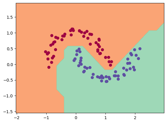
Look at that! It's not a straight line! It is a beautiful non-linear curve that perfectly hugs the two moons. The neural net has "understood" the geometry of the data.
Conclusion
I started with a blank jupyter notebook. I defined a Value object that wraps a single number. Taught that object how to add and multiply and crucially how to calculate its own local derivative. I chained these objects together into Neurons, Layers and MLPs.
Then, I threw a complex, non-linear classification problem at it. Defined a loss function and then just let the gradients flow.
The result is a working Deep Neural Network.
This zdravkograd engine is mathematically, "exactly" what PyTorch is. PyTorch uses Tensors (arrays) instead of scalars for efficiency, and it uses C++/CUDA for speed, but the soul of the software is identical. It is just a DAG (Directed Acyclic Graph) of operations that knows how to chain rule its way backwards.
I have fully demystified deep learning. It is not magic, it is just gradients and chain rule all the way down.
Thank you for reading :)