This is the continuation of the implementation of sequentia, in part 1 I implemented the bigram language model. I implemented is both using counts as well as a super simple neural network that is a single linear layer. The way I approached it was by just looking at the single previous character and predicted the distribution for the character that would go next, I did this by taking counts and normalising them into probabilities so that each row in our table summed up to 1. This is fine if you only have 1 character of previous context, it works and it's approachable. The problem with this model is that the predictions are not very good because you only take one character of context, so the model didn't produce very name like sounding things.
The problem with this approach though is that if I were to take more context into account when predicting the next character in a sequence things quickly blow up, and the size of our table (see below) that we had grows, in fact it would grow exponentially with the length of the context:
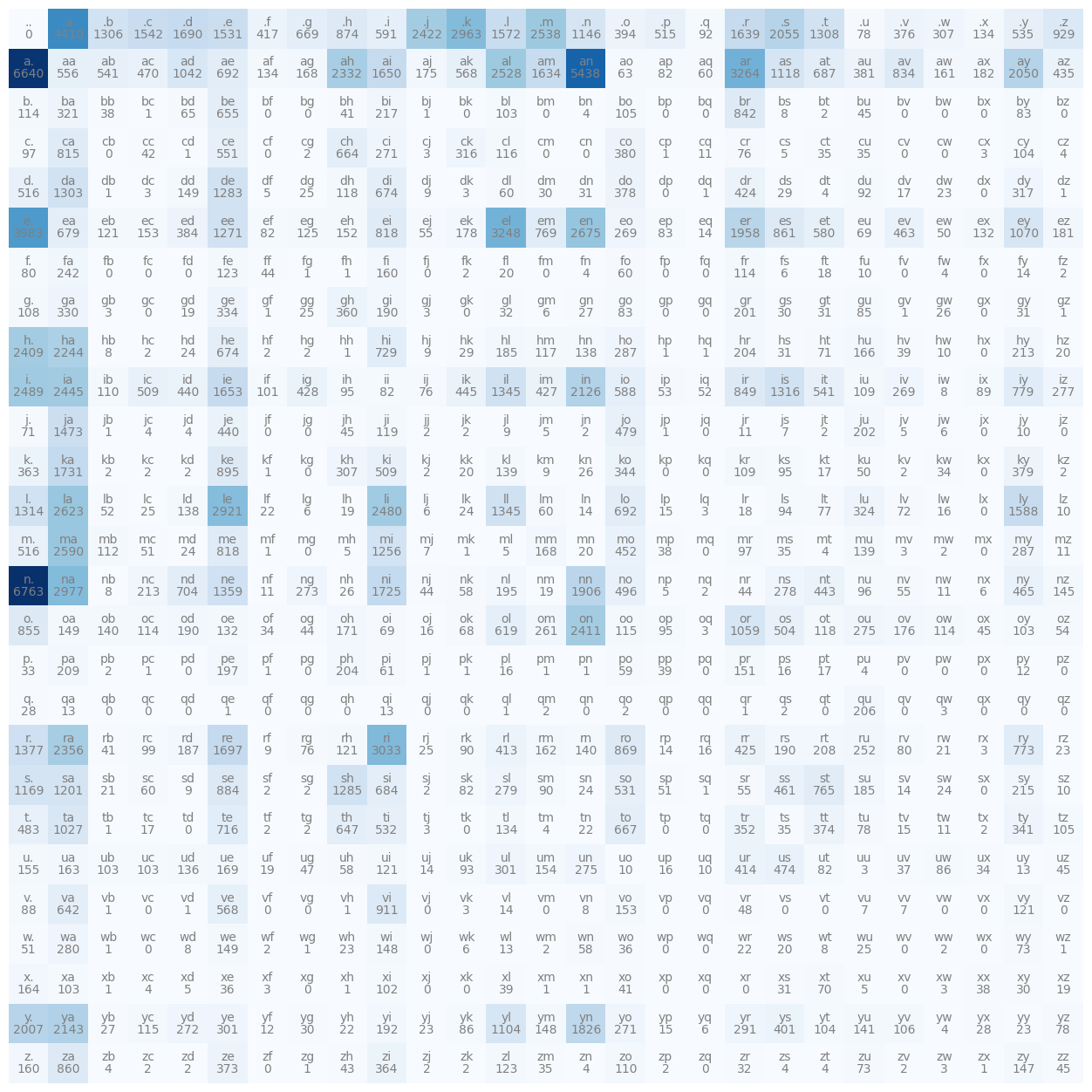
This is because if we only take a single character at a time thats 27 possibilities of context, but if we take 2 characters in a pass and try to predict the third one, suddenly the number of rows in the matrix is 27x27, so there's 729 possibilities for what could have come in the context. If we take 3 characters as the context then we would have around 20 thousand possibilities, and so that's just way too many rows to have in our matrix, the whole thing just kind of explodes and doesn't work very well.
That's why now I'm going to implement a multilayer perceptron model to predict the next character in a sequence and the modelling approach that I'm going to adopt follows this paper: A Neural Probabilistic Language Model. This isn't the very first paper that proposed the use of MLPs or neural networks to predict the next character or token in a sequence but it's definitely one that was very influencial around its time. So first I'll have a look and understand it and then I'll implement it.
Now, this paper has 19 pages so I'm not going to go into full details here but I recommend you read it. In the introduction they describe the exact same problem I just described and then to address it they propose the following model.
By the way, keep in mind that I am building a character level language model so I'm working on the level of characters, in this paper however they have a vocabulary of 17,000 possible words and they instead build a word level language model, I'm going to still stick with the characters but take the same modelling approach.
They propose to take every one of those 17,000 words and associate to each word a 30 dimensional feature vector, so every word is now embedded into a 30 dimensional space. So we have 17,000 points/vectors in a 30 dimensional space, you might imagine that it is very crowded as that is a lot of points for a very small space. In the beginning these words are initialised completely randomly, they are spread out at random, but then these embeddings of these words get tuned using backprop. So during the course of training this neural network these points or vectors are basically going to move around in this space and you might imagine for example that words that have a similar meaning or are synonyms of each other might end up in a very similar part of the space. Conversely, words that have very different meanings would end up being far from each other.
Otherwise, the modelling approach is identical to ours, they are using a multilayer neural network to predict the next word given the previous words and to train the neural network they are maximising the log likelihood of the training data just like I did in the previous part. Let's go over a concrete example of their intuition from the paper.
Why does it work?
Suppose for example that you are trying to predict:
A dog was running in a ______.
Suppose also that that exact phrase has never occurred in the training data and here we are at test time (later, so when the model is deployed somewhere) and it's trying to make a sentence and because it's never encountered this exact phrase in the training set we are out of distribution. Essentially, we don't have any fundamental reason to suspect what might come next. However, this approach allows us to get around that because maybe you didn't see the exact phrase "A dog was running in a ______" but maybe you have seen similar phrases like for example "The dog was running in a ______" and maybe the network has learnt that "A" and "The" are frequently interchangeable with each other. So maybe it took the embedding for "A" and the embedding for "The" and put them nearby each other in the space, so we can like this transfer knowledge through these embeddings and we can generalise in that way.
Similarly, the network could know that cats and dogs are animals and they co-occur in lots of contexts and so even though it hasn't seen some exact phrase we can transfer knowledge through the embedding space and generalise to novel scenarios.
Let's now go down a little to this diagram of the neural network that appears in the paper:
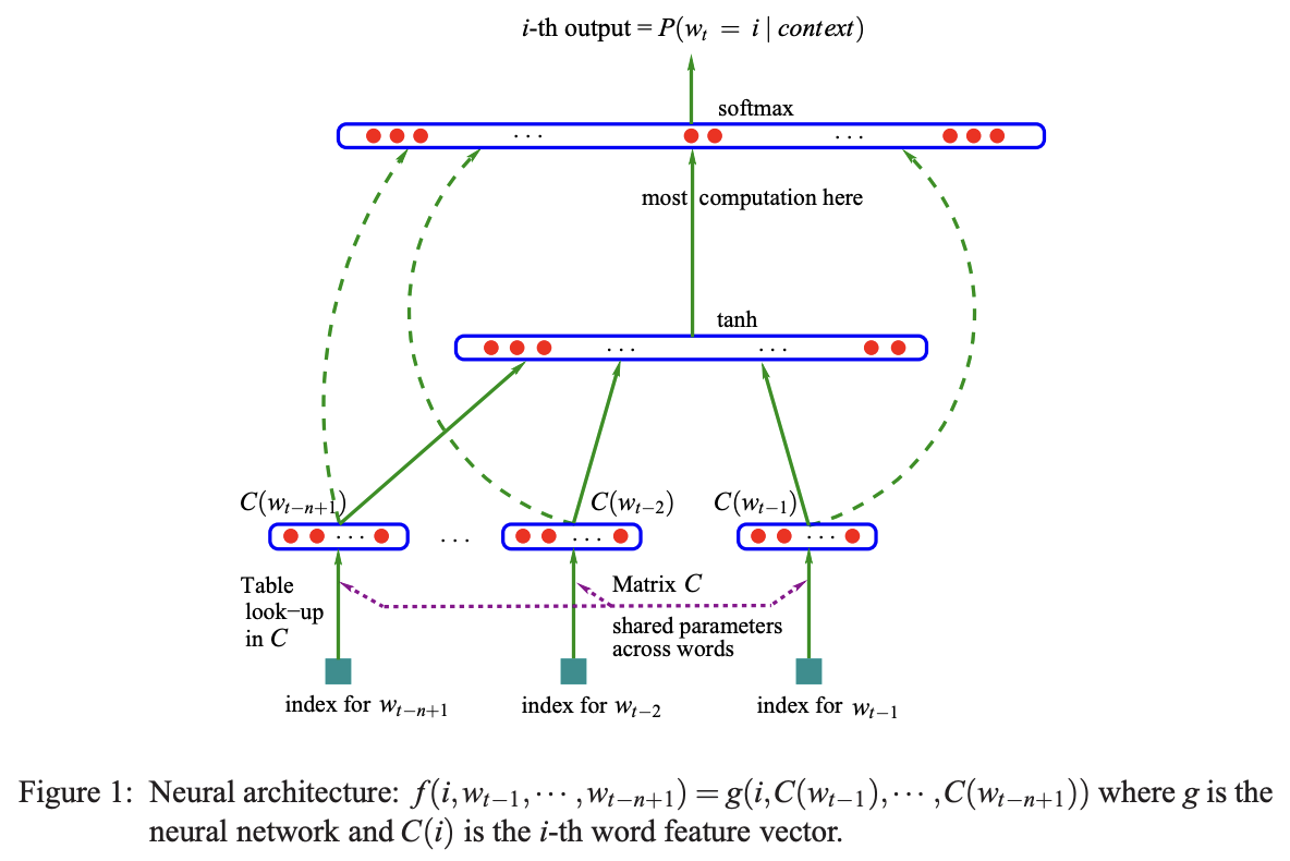
They have a nice diagram here and in this example we are taking 3 previous words and we are trying to predict the 4th word in a sequence. These 3 previous words (coming from our vocabulary of 17,000 possible words), every one of these are basically the index of the incoming word, because there are 17,000 this will be an integer between 0 and 16,999. There is also this lookup table that they call C, this lookup table is a matrix that is 17,000 by 30, so every index is plucking out a row of this embedding matrix so that each index is converted into the 30 dimensional vector that corresponds to the embedding vector for that word.
So at the bottom we have the input layer of 30 neurons for 3 words making up 90 neurons in total. They also state that this matrix C is shared across all these words. So we are always indexing into the same matrix C over and over for each one of these words.
Next up is the hidden layer of this network, the size of this layer is a hyperparameter (a configuration setting chosen before training begins, controlling the learning process itself) it is a design choice up to the designer of the neural net, this can be as large as you'd like or as small as you'd like. I will go over multiple choices of the size of this hidden layer and evaluate how well each one works.
So say there were 100 neurons here, all of them would be fully connected to the 90 numbers that make up the initial 3 input words, so this would be a fully connected layer. Then there is a tanh nonlinearity and then there's this output layer and because there are 17,000 possible words that could come next, this layer has 17,000 neurons and all of them are fully connected to all of the neurons in the hidden layer. So there's a lot of parameters here because there's a lot of words, most computation is here as this is the expensive layer.
So there are 17,000 logits here so on top of there we have this softmax layer, which I used in part 1, so every one of these logits is exponentiated and then everything is normalised to sum to 1 so that we have a nice probability distribution for the next word in the sequence.
Now of course during training we actually have the label, we have the identity of the next word in the sequence. That word, or its index is used to pluck out the probability of that word and then we are maximising the probability of that word with respect to the parameters of this neural net. So the parameters are the weights and biases of this output layer, the weights and biases of this hidden layer and the embedding lookup table C, all of that is optimised using backpropogation. (Ignore the dashed arrows in the image, it represents a variation of a neural net that I'm not going to explore now)
So that's the setup and now let's implement it!
Ok so I'm starting a brand new jupyter notebook for this part.
import torch
import torch.nn.functional as F
import matplotlib.pyplot as plt
%matplotlib inline
Starting off by importing PyTorch as well as matplotlib so I can create figures.
words = open('names.txt', 'r').read().splitlines()
words[:8]
Then I'm reading all the names into a list of words like I did before and for now going to be using the first 8, keep in mind that there are around 32,000 in total.
chars = sorted(list(set(''.join(words))))
stoi = {s:i+1 for i,s in enumerate(chars)}
stoi['.'] = 0
itos = {i:s for s,i in stoi.items()}
print(itos)
Here I am building out the vocabulary of characters and all the mappings from the characters as strings to integers and vice versa.
Now the first thing that we want to do is we want to compile the dataset for the neural network.
# build the dataset

block_size = 3
X, Y = [], []
for w in words[:5]:
    print(w)
    context = [0] * block_size
    for ch in w + '.':
        ix = stoi[ch]
        X.append(context)
        Y.append(ix)
        print(''.join(itos[i] for i in context), '--->', itos[ix])
        context = context[1:] + [ix]

X = torch.tensor(X)
Y = torch.tensor(Y)
So this is the code used for the dataset creation, let's run it and then I'll explain how it works:
emma
... ---> e
..e ---> m
.em ---> m
emm ---> a
mma ---> .
olivia
... ---> o
..o ---> l
.ol ---> i
oli ---> v
liv ---> i
ivi ---> a
via ---> .
ava
... ---> a
..a ---> v
.av ---> a
ava ---> .
isabella
... ---> i
..i ---> s
.is ---> a
isa ---> b
sab ---> e
...
sop ---> h
oph ---> i
phi ---> a
hia ---> .
So first I defined something called block_size this is essentially the context length of how many characters do we take to predict the next one? In the example diagram from the paper they are using 3 characters to predict the 4th one so we have a block size of 3. Then I build out the X and Y, the X are the inputs to the neural net and the Y are the labels for each example inside X. Then I'm iterating over the first 5 words, for now this is just for efficiency and later on I'll use the entire training set. Then I'm printing a word, 'emma', and then I'm showing the 5 examples that we can generate out of the single word emma. So when we are given the context of ... the first character in the sequence is e, in the second context the label is m and so on.
The way this is built out is first we start with a padded context of just 0 tokens, then I iterate over all the characters, I get the character in a sequence and I build out the arrat Y of this current character and the array X which stores the current running context, then I print everything and finally I crop the context and enter the new character in the sequence, so this is kind of like a rolling window of context.
Now we can change the block_size to like 4 and we get this:
emma
.... ---> e
...e ---> m
..em ---> m
.emm ---> a
emma ---> .
olivia
.... ---> o
...o ---> l
..ol ---> i
.oli ---> v
oliv ---> i
livi ---> a
ivia ---> .
ava
.... ---> a
...a ---> v
..av ---> a
.ava ---> .
isabella
.... ---> i
...i ---> s
..is ---> a
.isa ---> b
isab ---> e
...
.sop ---> h
soph ---> i
ophi ---> a
phia ---> .
And in this case we would be predicting the 5th character given the previous 4. I'll use 3 as the block_size so that I have something similar to what they use in the paper.
So the dataset right now looks as follows:
X.shape, X.dtype, Y.shape, Y.dtype(torch.Size([32, 4]), torch.int64, torch.Size([32]), torch.int64)From these 5 words, I have created a dataset of 32 examples, each input to the neural net is 3 integers and we also have a label that is also an integer Y. So X looks like this:
tensor([[ 0,  0,  0,  0],
        [ 0,  0,  0,  5],
        [ 0,  0,  5, 13],
        [ 0,  5, 13, 13],
        [ 5, 13, 13,  1],
        [ 0,  0,  0,  0],
        [ 0,  0,  0, 15],
        [ 0,  0, 15, 12],
        [ 0, 15, 12,  9],
        [15, 12,  9, 22],
        [12,  9, 22,  9],
        [ 9, 22,  9,  1],
        [ 0,  0,  0,  0],
        [ 0,  0,  0,  1],
        [ 0,  0,  1, 22],
        [ 0,  1, 22,  1],
        [ 0,  0,  0,  0],
        [ 0,  0,  0,  9],
        [ 0,  0,  9, 19],
        [ 0,  9, 19,  1],
        [ 9, 19,  1,  2],
        [19,  1,  2,  5],
        [ 1,  2,  5, 12],
        [ 2,  5, 12, 12],
        [ 5, 12, 12,  1],
...
        [ 0,  0, 19, 15],
        [ 0, 19, 15, 16],
        [19, 15, 16,  8],
        [15, 16,  8,  9],
        [16,  8,  9,  1]])
These are the individual examples and then Y are the labels:
tensor([ 5, 13, 13,  1,  0, 15, 12,  9, 22,  9,  1,  0,  1, 22,  1,  0,  9, 19,
         1,  2,  5, 12, 12,  1,  0, 19, 15, 16,  8,  9,  1,  0])
So now given this let's now write a neural network that takes these X's and predicts the Y's.
First let's build the embedding lookup table C. So we have 27 possible characters and we are going to embed them in a lower dimensional space, in the paper for example they have 17,000 words and they embed them in a space as small as 30, so they cram 17,000 words into a 30 dimensional space. In our case we have only 27 possible characters so let's cram them into something as small as a 2 dimensional space. C = torch.randn((27, 2)) so this lookup table will be random numbers, we'll have 27 rows and 2 columns, so each one of those 27 characters will have a 2 dimensional embedding.
tensor([[ 0.1337, -0.3022],
        [-1.3790,  0.5350],
        [-0.4888,  0.3871],
        [-1.0085, -0.3628],
        [-0.7620,  0.2085],
        [-2.1093, -0.5866],
        [-0.3420, -0.5095],
        [-0.2952,  1.9254],
        [-1.4044,  0.9889],
        [ 0.5346, -0.5347],
        [-0.2993,  1.2175],
        [-2.3203, -1.8098],
        [-0.4861,  0.1701],
        [-1.6238,  0.3501],
        [ 2.7832,  2.1153],
        [ 0.2209, -0.1851],
        [ 1.0563,  0.1075],
        [ 0.4634,  0.8870],
        [-0.3711,  1.1748],
        [-0.4258,  1.7453],
        [-0.4970, -0.2934],
        [ 0.9061,  1.1547],
        [ 1.4147,  0.6171],
        [-2.0147,  0.8542],
        [-0.3040,  0.3283],
        [ 0.0795, -1.3960],
        [-0.5026,  0.0559]])
So that's our matrix C of embeddings in the beginning initialised randomly. Now before we embed all of the integers inside the input X using this lookup table C let me actually just try to embed a single lookupu integer like let's say 5, so we get a sense of how this works. One way this works is we can take the C and index into row 5 C[5 and that gives us tensor([-0.5042, 0.8381]) a vector, the fifth row of C, this is one way to do it. The other way, that was actually used in part 1 of sequentia, that was seemingly different but actually identical. Essentially, I took the integers and used one hot encoding to first encode them. F.one_hot(5, num_classes=27), so that's the 26 dimensional vector of all 0s except the 5th bit is turned on. Now this actually doesn't work:
---------------------------------------------------------------------------
TypeError                                 Traceback (most recent call last)
Cell In[17], line 1
----> 1 F.one_hot(5, num_classes=27)

TypeError: one_hot(): argument 'input' (position 1) must be Tensor, not int
The reason is that this input wants to be a torch.tensor, F.one_hot(torch.tensor(5), num_classes=27) now this outputs the correct one hot vector:
tensor([0, 0, 0, 0, 0, 1, 0, 0, 0, 0, 0, 0, 0, 0, 0, 0, 0, 0, 0, 0, 0, 0, 0, 0,
        0, 0, 0])
The fifth dimension is 1 and the shape of this is 27. So now if we take this one hot vector and we multiply it by C then what would you expect to get?
Well firstly, we should expect to get an error:
---------------------------------------------------------------------------
RuntimeError                              Traceback (most recent call last)
Cell In[19], line 1
----> 1 F.one_hot(torch.tensor(5), num_classes=27) @ C

RuntimeError: expected m1 and m2 to have the same dtype, but got: long long != float
The error might be a little confusing but the problem here is that one hot, the data type of it is long:
F.one_hot(torch.tensor(5), num_classes=27).dtypetorch.int64It's a 64 bit integer but our C is a float tensor, PyTorch doesn't know how to multiply an int with a float so we have to explicitly cast the one hot vector to a float so that we can multiply, and once we do that we get this:
tensor([-0.5042, 0.8381])The output here is actually identical, this is because of the way matrix multiplication here works. This tells me that the first part of the diagram up above, the first piece of it (the embedding of the integer) can either be thought of the integer indexing into a lookup table C but equivalently we can also think of this little piece here as the first layer of this bigger neural net. This layer has neurons that have no nonlinearity, theres no tanh, and their weight matrix is just C, then we are encoding integers into one hot and feeding them into a neural net and this first layer basically embeds them.
So those are two equivalent ways of doing the same thing, I'm just going to index, C[5], becuase its much much faster and discard the latter interpretation of one hot inputs into neural nets.
Embedding a single integer like 5 is easy enough, we can simply ask PyTorch to retrieve the row of index 5 of C, but how do we simultaneously embed all of these 32x3 integers stored in array X. Luckily PyTorch indexing is fairly flexible and quite powerful, we can actually index using lists, for example we can the rows 5, 6 and 7 like this C[[5, 6, 7]] and it will just work:
tensor([[-0.5042,  0.8381],
        [ 1.7272,  0.5446],
        [-0.6218,  1.0026]])
So we can index with a list, it also doesn't have to just be a list we can actually index with a tensor of integers: C[torch.tensor([5, 6, 7])], we can also repeat row 7 for example and retrieve it multiple times C[torch.tensor([5, 6, 7, 7, 7, 7])]:
tensor([[-0.5042,  0.8381],
        [ 1.7272,  0.5446],
        [-0.6218,  1.0026],
        [-0.6218,  1.0026],
        [-0.6218,  1.0026],
        [-0.6218,  1.0026]])
So here we are indexing with a one dimensional tensor of integers but we can also index with multi dimensional tensor of integers meaning we can simply do C[X] and it will just work:
tensor([[[-1.5906,  2.1496],
         [-1.5906,  2.1496],
         [-1.5906,  2.1496],
         [-1.5906,  2.1496]],

        [[-1.5906,  2.1496],
         [-1.5906,  2.1496],
         [-1.5906,  2.1496],
         [-0.5042,  0.8381]],

        [[-1.5906,  2.1496],
         [-1.5906,  2.1496],
         [-0.5042,  0.8381],
         [-0.7761, -0.4062]],

        [[-1.5906,  2.1496],
         [-0.5042,  0.8381],
         [-0.7761, -0.4062],
         [-0.7761, -0.4062]],

        [[-0.5042,  0.8381],
         [-0.7761, -0.4062],
         [-0.7761, -0.4062],
         [ 0.3950, -0.4444]],
...

        [[-0.6436, -0.4006],
         [-0.1759, -0.8072],
         [-1.3593,  1.4689],
         [ 0.3950, -0.4444]]])
And the shape of this is torch.Size([32, 3, 2]), so 32x3 which is the original shape and now for every one of those 32x3 integers we've retrieved the embedding vector as well. So for example, X[13, 2] the 2nd dimension at index 13 is: tensor(1) the integer 1 and so if we do C[X] and then we index into C[X][13, 2] then we get the embedding tensor([ 0.7906, -0.3438]) and you can verify that at C[1] which is the integer at that location is indeed tensor([ 0.7906, -0.3438]) equal to that. So basically, long story short, PyTorch indexing is awesome and to embed simultaneously all of the integers in X we can simply do emb = C[X] and that is our embedding.
Now let's construct the hidden layer. W1 will be the weights which will be initialised randomly and the number of inputs to this layer is going to be 3x2 because we have 2 dimensional embeddings and we have 3 of them, so the number of inputs is 6, and the number of neurons in this layer is a variable that is up to us, let's use 100 as an example. Then biases b will also be initialised randomly as an example and we will just need 100 of them.
W1 = torch.randn((6, 100))
b1 = torch.randn((100))
Normally, we would take the input, in this case that's embedding and we would like to multiply it with these weights and then add the biases, this is roughly what we want to do, but the problem here is that these embeddings are stacked up in the dimensions of this input tensor, so this matrix multiplication emb @ W1 + b1 will not work because emb is a shape 32x3x2 and it cannot be multilplied by 6x100, so somehow we need to concatenate the inputs so that we can do that matrix multiplication. So how do we tranform our 32x3x2 into a 32x6 so that we can actually perform the multiplication over here.
There are usually many ways of implementing anything you would like to do in torch, some of them will be faster, better, shrter etc. and this is because torch is a very large library and its got lots and lots of functions. One of the things that we can do is torch.cat and this concatenates the given sequence of tensors in a given dimension.
So again we want to retrieve those three parts and concatenate them, emb[:, 0, :] this plucks out all of the 32 embeddings of just the first word, we want that guy, we want this guy: emb[:, 1, :] as well as this guy: emb[:, 2, :], these are the three pieces individually. Then we treat this as a sequence and we torch.cat on that sequence, but then we also have to tell it along which dimension to concatenate, so in this case all of these are 32x2 and we want to not concat over the first dimension the 32 but rather the second one, so its index would be 1.
tensor([[ 0.4444, -0.1867,  0.4444, -0.1867,  0.4444, -0.1867],
        [ 0.4444, -0.1867,  0.4444, -0.1867,  1.6435,  1.8505],
        [ 0.4444, -0.1867,  1.6435,  1.8505,  0.4650, -0.0786],
        [ 1.6435,  1.8505,  0.4650, -0.0786,  0.4650, -0.0786],
        [ 0.4650, -0.0786,  0.4650, -0.0786,  0.7906, -0.3438],
        [ 0.4444, -0.1867,  0.4444, -0.1867,  0.4444, -0.1867],
        [ 0.4444, -0.1867,  0.4444, -0.1867, -0.8392, -0.6142],
        [ 0.4444, -0.1867, -0.8392, -0.6142, -0.9680,  0.3780],
        [-0.8392, -0.6142, -0.9680,  0.3780,  0.0479,  0.8135],
        [-0.9680,  0.3780,  0.0479,  0.8135, -1.1759,  1.5259],
        [ 0.0479,  0.8135, -1.1759,  1.5259,  0.0479,  0.8135],
        [-1.1759,  1.5259,  0.0479,  0.8135,  0.7906, -0.3438],
        [ 0.4444, -0.1867,  0.4444, -0.1867,  0.4444, -0.1867],
        [ 0.4444, -0.1867,  0.4444, -0.1867,  0.7906, -0.3438],
        [ 0.4444, -0.1867,  0.7906, -0.3438, -1.1759,  1.5259],
        [ 0.7906, -0.3438, -1.1759,  1.5259,  0.7906, -0.3438],
        [ 0.4444, -0.1867,  0.4444, -0.1867,  0.4444, -0.1867],
        [ 0.4444, -0.1867,  0.4444, -0.1867,  0.0479,  0.8135],
        [ 0.4444, -0.1867,  0.0479,  0.8135,  0.3600, -1.0378],
        [ 0.0479,  0.8135,  0.3600, -1.0378,  0.7906, -0.3438],
        [ 0.3600, -1.0378,  0.7906, -0.3438,  2.0007,  0.6971],
        [ 0.7906, -0.3438,  2.0007,  0.6971,  1.6435,  1.8505],
        [ 2.0007,  0.6971,  1.6435,  1.8505, -0.9680,  0.3780],
        [ 1.6435,  1.8505, -0.9680,  0.3780, -0.9680,  0.3780],
        [-0.9680,  0.3780, -0.9680,  0.3780,  0.7906, -0.3438],
...
        [ 0.4444, -0.1867,  0.3600, -1.0378, -0.8392, -0.6142],
        [ 0.3600, -1.0378, -0.8392, -0.6142,  1.0230, -0.0592],
        [-0.8392, -0.6142,  1.0230, -0.0592, -0.7218, -0.3401],
        [ 1.0230, -0.0592, -0.7218, -0.3401,  0.0479,  0.8135],
        [-0.7218, -0.3401,  0.0479,  0.8135,  0.7906, -0.3438]])
This is our concatenated result and its shape is 32x6, exactly as we'd like. The issue is that this code above is kind of ugly because it is not genaralisable, if we change the block_size it would not work. Torch comes to rescue again because there is a function called unbind which removes a tensor dimension and returns a tuple of all slices along a given dimension already without it. So when we call torch.unbind(emb) and pass in the 2nd dimension it gives us a list of tensors exactly equivalent to what we had previously. So the neater version of the code is:
torch.cat(torch.unbind(emb, 1), 1)Now it doens't matter if we have block_size 3, 5, 10 or anything this will just work. So this is one way to do it.
However, it turns out that in this case there's actually a significantly better and more efficient way!
Let's create an array here of elements from 0 to 17, a = torch.arange(18):
tensor([ 0, 1, 2, 3, 4, 5, 6, 7, 8, 9, 10, 11, 12, 13, 14, 15, 16, 17])and the shape of this is torch.Size([18]), it turns out that we can very quickly re represent this as different sized n dimensional tensors, we can do this by calling a.view(), and we can say that this shouldn't be a single vector of 18 but rather a 2x9 vector: a.view(2, 9):
tensor([[ 0,  1,  2,  3,  4,  5,  6,  7,  8],
        [ 9, 10, 11, 12, 13, 14, 15, 16, 17]])
or alternatively a 9x2 tensor: a.view(9, 2):
tensor([[ 0,  1],
        [ 2,  3],
        [ 4,  5],
        [ 6,  7],
        [ 8,  9],
        [10, 11],
        [12, 13],
        [14, 15],
        [16, 17]])
as long as the total number multiplies to be the same this will just work and in PyTorch this view() operation is extremely efficient and the reason for that is that in each tensor there is something called storage(). The storage is just the numbers as a 1 dimensional vector, always, this is how this tensor is represented in the computer's memory. When we call the view operation we are manipulating some of the attributes that dictate how this 1 dimensional sequence is interpreted to be an n dimensional tensor. So when we call the view operation no memory is being changed, copied, moved or created, the storage is identical, but when we call view some of the internal attributes of this tensor are being manipulated and changed. In particular there's something called storage offset, strides and shapes and those are manipulated so that this 1 dimensional sequence of bytes is seen as different n dimensional arrays.
There is a blog post that goes in depth with the PyTorch internals that is a good read but for now all that we need to know is that view() is an extremely efficient operation.
So we just need to ask PyTorch to view our emb as a 32x6 like this: emb.view(32, 6) and the way that this does it just so happens to be that each two numbers get stacked the same way the concatenation method does it too, and we can verify that this gives the exact same result with this:
torch.cat(torch.unbind(emb, 1), 1) == emb.view(32, 6)which spits out
tensor([[True, True, True, True, True, True],
        [True, True, True, True, True, True],
        [True, True, True, True, True, True],
        [True, True, True, True, True, True],
        [True, True, True, True, True, True],
        [True, True, True, True, True, True],
        [True, True, True, True, True, True],
        [True, True, True, True, True, True],
        [True, True, True, True, True, True],
        [True, True, True, True, True, True],
        [True, True, True, True, True, True],
        [True, True, True, True, True, True],
        [True, True, True, True, True, True],
        [True, True, True, True, True, True],
        [True, True, True, True, True, True],
        [True, True, True, True, True, True],
        [True, True, True, True, True, True],
        [True, True, True, True, True, True],
        [True, True, True, True, True, True],
        [True, True, True, True, True, True],
        [True, True, True, True, True, True],
        [True, True, True, True, True, True],
        [True, True, True, True, True, True],
        [True, True, True, True, True, True],
        [True, True, True, True, True, True],
...
        [True, True, True, True, True, True],
        [True, True, True, True, True, True],
        [True, True, True, True, True, True],
        [True, True, True, True, True, True],
        [True, True, True, True, True, True]])
we see it in this representation because it is an element-wise eqauls, it is clearly visible that they are all True.
Long story short, I can actually come here and simply use it:
emb.view(32, 6) @ W1 + b1tensor([[-1.4762, -0.1819, -1.9316, ..., -1.1295, 0.9217, 0.1658],
[-3.4858, -1.4528, -1.3809, ..., -3.0438, 0.9032, -5.8463],
[-1.7364, -0.4168, -3.1396, ..., 0.8445, -3.1651, 1.1465],
...,
[ 1.9684, 0.6379, -1.3668, ..., 1.5785, -0.2257, 4.3608],
[-3.0535, -0.2721, -2.2716, ..., -3.8546, 4.3116, -1.6676],
[-0.1189, 1.7893, -1.8674, ..., -0.3386, -0.5712, -1.4834]])This multiplication now works and gives us the hidden states that we are after. I'll store the result in h and h.shape is now torch.Size([32, 100]), the 100 dimensional activations for every one of our 32 examples.
Two things that I would like to update, number 1 is for this line h = emb.view(32, 6) @ W1 + b1 let's not use 32 as that is hardcoded, let's instead use emb.shape[0] that way this would work for any size of our embeddings. Alternatively, we can also just use -1, in this case PyTorch would infer what this should be, this is because the number of elements must be the same and if we say that the other number is 6 PyTorch would derive that this must be 32 in this case or whatever else it is if emb is of different size.
h = torch.tanh(emb.view(-1, 6) @ W1 + b1)Also I will add that tanh to calculate h, this way the numbers would be between -1 and 1 because of the tanh, and that is basically our hidden layer complete.
Actually, one last thing that I want to point out is to do with the plus between the weights and the biases. It is vital to make sure that teh broadcasting will do what we need it to do.
(emb.view(-1, 6) @ W1).shape
# torch.Size([32, 100])

b1.shape
# torch.Size([100])
The shape of the first part is 32x100 and b1's shape is 100, so the addition will broadcast these two. In particular we have:
# 32, 100
#     100

# 32, 100
#  1, 100
So 32x100 broadcasting to 100, it aligns on the right, create a fake dimension to make it a 1x100 row vector and then it will copy vertically for every one of these rows of 32 and do an element-wise addition. In this case, the correct thing will be happening because the same bias vector will be added to all the rows of our matrix, which is what we'd like to happen but its still always good practise to make sure and verify these things.
Finally, let's create the final layer, so let's create W2 and b2:
W2 = torch.randn((100, 27))
b2 = torch.randn((27))
The input now is 100 and the output number of neurons will be 27 because we have 27 possible characters that could come next. That means the biases will also be 27. Therefore, the logits, which are the output for this neural net will be logits = h @ W2 + b2. logits.shape is torch.Size([32, 27]) and the logits look like this:
tensor([[ 9.2186e-01,  7.8329e+00,  8.9391e+00,  1.3031e+01,  1.0261e+01,
         -9.3190e-01, -1.5131e-01, -4.9145e+00,  7.9880e+00, -5.0248e+00,
         -1.4477e+01, -3.4141e+00,  2.4284e+00,  4.3457e+00,  6.5878e+00,
         -4.6248e+00,  1.1070e+01, -4.8569e+00,  6.9940e-01, -1.0852e-01,
          2.8623e+01,  8.8996e+00, -3.1435e+00,  5.3032e+00,  8.2720e+00,
          6.8641e+00,  2.9711e+00],
        [ 1.5082e+00,  6.3957e+00,  1.0389e+01,  9.1203e+00,  6.0596e+00,
          4.4575e+00, -3.0974e+00, -8.4399e+00,  9.4483e+00, -5.8028e+00,
         -1.6847e+01, -2.3563e+00, -1.3673e+00,  9.6829e+00,  6.6244e+00,
         -1.0214e+00,  6.1324e+00, -8.3729e+00, -1.2231e-01, -8.1913e-01,
          2.4516e+01,  7.5482e+00, -2.0436e+00,  7.7832e+00,  4.7609e+00,
          7.5728e+00,  4.2434e+00],
        [-3.0164e+00, -4.3449e-01,  2.9850e+00,  1.9821e+01,  1.2524e+01,
         -9.2205e+00,  1.7786e+00,  2.8449e+00,  4.9969e+00,  4.2911e-01,
         -1.8727e+01, -9.2163e-01,  7.3207e+00,  1.0234e+00,  9.1815e+00,
         -1.4192e+01,  1.2777e+01, -8.1739e+00,  5.9195e+00,  6.0474e+00,
          1.8890e+01,  4.7528e+00, -1.1540e+01,  2.6521e-01,  8.8773e+00,
          5.7664e+00,  4.6899e+00],
        [ 5.6007e+00,  1.3426e+00, -4.2855e+00,  1.1434e+01,  1.1768e+01,
         -1.2407e+01,  5.4088e+00, -5.0530e+00, -5.1155e+00, -1.1577e+01,
         -6.3449e+00, -3.9113e+00,  3.1780e+00, -4.5127e+00,  1.9136e+00,
         -9.5595e+00,  1.4481e+01, -6.3205e+00, -3.5052e+00,  7.4086e+00,
          1.2277e+01, -5.9215e+00,  5.8912e+00,  3.4803e+00,  5.0781e+00,
          7.4746e+00,  4.0147e-01],
        [ 2.2878e+00,  5.2810e+00,  3.9140e+00,  5.6183e+00,  4.8376e+00,
...
         -2.9292e+00, -4.8113e+00,  2.3394e+00, -1.1899e+01, -1.1731e+01,
          5.7530e+00,  4.1429e-01, -6.8187e-01, -1.8771e+00, -3.5143e+00,
         -9.2754e+00,  9.9399e+00, -2.5397e-01, -1.0469e+01, -7.2643e+00,
          6.1939e+00, -6.5458e+00,  9.3165e+00,  8.9809e+00,  6.7254e+00,
          1.8464e+01, -7.8833e+00]])
Now, exactly as we did in part 1, we take these logits and we first exponentiate them to get our "fake" counts: counts = logits.exp(). Then we need to normalise them into a probability:
prob = counts / counts.sum(1, keepdim=True)prob.shape is now torch.Size([32, 27]) and every row of prob prob[0].sum() sums to tensor(1.), so it's normalised, now we have the probabilities. Now we have the actual layer that comes next and that comes from this array Y which we created during the dataset creation. So Y is the last piece which is the identity of the next character in the sequence that we'd like to now predict.
So, just like in part 1, we need to index into the rows of prob and in each row we'd like to pluck out the probability assigned to the correct character that's given in Y. First, we have torch.arange(32) which is our iterator over number from 0-31 and then we can index into prob in the following way:
prob[torch.arange(32), Y]This gives the current probabilities assigned by this neural network with the current setting of its weights to the correct character in the sequence.
tensor([1.4601e-13, 3.6158e-07, 4.9148e-09, 1.6047e-06, 1.8780e-05, 3.6353e-15,
        4.5551e-09, 1.2741e-09, 1.0886e-10, 1.3372e-09, 1.6603e-06, 2.7156e-03,
        9.3519e-10, 2.9309e-12, 5.1150e-08, 6.9192e-09, 2.4369e-15, 1.8135e-03,
        1.9740e-07, 1.7723e-02, 6.1448e-09, 5.5966e-10, 4.8843e-08, 9.8783e-08,
        1.0280e-11, 3.3263e-13, 7.3331e-12, 8.1707e-02, 8.7775e-04, 3.4055e-07,
        2.6619e-04, 2.2750e-05])
It is visible to see that this looks absolutely terrible currently, some of these are extremely unlikely but of course we have't trained the neural network yet so this will improve and ideally all of these numbers of course are 1 because then we are correctly predicting the next character.
Now, just as in part 1, we take these probs, we want to look at the log probability and then we want to look at the average of those and then the negative of it to create the negative log likelihood loss:
loss = -prob[torch.arange(32), Y].log().mean()which currently sits at: tensor(17.5572), this is the loss that we'd like to minimise to get the network to predict the correct character in the sequence.
Ok, so to rewrite everything to make it a little more respectable, here we have our dataset.
X.shape, Y.shape(torch.Size([32, 3]), torch.Size([32]))Here are all the parameters that we defined and now using a generator to make it reproducible and also clustered all the parameters into a single list so that it is easy to count them.
g = torch.Generator().manual_seed(2147483647)
C = torch.randn((27, 2), generator=g)
W1 = torch.randn((6, 100), generator=g)
b1 = torch.randn((100), generator=g)
W2 = torch.randn((100, 27), generator=g)
b2 = torch.randn((27), generator=g)
parameters = [C, W1, b1, W2, b2]
This is the code I used to count them and in total we have 3481 parameters.
sum(p.nelement() for p in parameters)And this is the forward pass and after running it I arrive at a single number, the loss, that is currently expressing how well this neural network works with the current setting of parameters.
emb = C[X]
h = torch.tanh(emb.view(-1, 6) @ W1 + b1)
logits = h @ W2 + b2
counts = logits.exp()
prob = counts / counts.sum(1, keepdim=True)
loss = -prob[torch.arange(32), Y].log().mean()
loss
The loss currently is tensor(17.7697).
Actually, it can be made even more respectable, in particular these lines above where we take the logits and we calculate a loss, we are not actually re-invneting the wheel here, this is just classification and many people use classification and that's why there is a functional.cross_entropy function in PyTorch to calcualte this much more efficiently. So we can just simply call F.cross_entropy and we can pass in the logits and the array of targets Y.
F.cross_entropy(logits, Y)and this calculates the exact same loss: tensor(17.7697).
So the more optimised code looks like this:
emb = C[X]
h = torch.tanh(emb.view(-1, 6) @ W1 + b1)
logits = h @ W2 + b2
loss = F.cross_entropy(logits, Y)
There are many good reasons to prefer this cross entropy function over rolling our own implementation like we did. I initially did it to learn what goes on behind the scenes but in practice that would never actually be done, why is that though?
When you use the cross entropy function, PyTorch will not actually create all those intermediate tensors because those would all be new tensors in memory. It clusters up all these operations and have fused kernels that very efficiently evaluate these expressions that are sort of clustered mathematical operations.
So the backward pass can be made much more efficient and not just because its a fused kernel but also analytically and mathematically its often a much more simpler backward pass to implement.
Number 2 is that this cross entropy function can also be significantly more numerically well behaved. Let me show you an example of how this works:
logits = torch.tensor([-2, -3, 0, 5])
counts = logits.exp()
probs = counts / counts.sum()
probs
Suppose we have these logits above and then we are taking the exponent of it and normalising it to sum to 1. So when logits takes on these values everything is well and good an we get a nice probability distribution:
tensor([9.0466e-04, 3.3281e-04, 6.6846e-03, 9.9208e-01])Now consider what happens when some of these logits take on more extreme values which happens during optimisation of the neural network. Suppose that some of these numbers grow to be very negative like the -2 becomes -100, in that case everything will come out fine:
tensor([0.0000e+00, 3.3311e-04, 6.6906e-03, 9.9298e-01])We still get probabilities that are well behaved and they sum to 1 and everything is great. However, because of the way the exp works, if we have very positive logits, like say the 5 becomes 100:
tensor([0., 0., 0., nan])Then we see that we start to run into trouble and we get "Not A Number" here, the reason for that is if we print the counts we see:
tensor([3.7835e-44, 4.9787e-02, 1.0000e+00, inf])they have an infinity there. So if you pass in a very negative number into exp we just get a very small number, which is fine, but if you pass in a very positive number then suddenly we run out of range in our floating point number that represents these counts. Basically, we are taking e and raising it to the power of 100 and that gives us inf because we've run out of dynamic range on this floating point number that is counts and so we cannot pass very large logits through this expression.
Now let me reset these numbers back to something reasonable:
logits = torch.tensor([-5, -3, 0, 5])
counts = logits.exp()
probs = counts / counts.sum()
probstensor([4.5079e-05, 3.3309e-04, 6.6903e-03, 9.9293e-01])The way PyTorch solves this is because of the normalisation you can actually offset logits by any arbitrary constant value that you want, so if I add 1 here:
logits = torch.tensor([-5, -3, 0, 5]) + 1then we actually get the exact same result
tensor([4.5079e-05, 3.3309e-04, 6.6903e-03, 9.9293e-01])or if I add 2 or subtract 3, any offset will produce the exact same probabilities. So because negative numbers are ok but positive numbers can actually overflow this exp what PyTorch does is it internally calculates the maximum value that occurs in the logits and it subtracts it. So in the case above it would subtract 5. Therefore, the greatest number in logits would become 0 and all the other numbers would become some negative numbers and then the result of this is always well behaved.
So again, there's many good reasons to use the cross entropy function, the forward pass can be much more efficient, the backward pass can be much more efficient and also things can be much more numerically well behaved.
Ok, so let's now set up the training of this neural net.
We have the forward pass:
emb = C[X]
h = torch.tanh(emb.view(-1, 6) @ W1 + b1)
logits = h @ W2 + b2
loss = F.cross_entropy(logits, Y)
Then we need the backward pass, first we need the gradients to be set to 0 and then we loss.backward() to populate those gradients.
for p in parameters:
    p.grad = None
loss.backward()
Once we get the gradients we can do the parameter update, so we loop over the parameters and nudge them, learning rate times p.grad.
for p in parameters:
    p.data += -0.1 * p.grad
Then we want to repeat this a few times and I'll also add a print statement so we can see the loss as this loops:
for _ in range(10):
    emb = C[X]
    h = torch.tanh(emb.view(-1, 6) @ W1 + b1)
    logits = h @ W2 + b2
    loss = F.cross_entropy(logits, Y)
    print(loss.item())

    for p in parameters:
        p.grad = None
    loss.backward()

    for p in parameters:
        p.data += -0.1 * p.grad
Now this will not suffice because we also need to loop over the parameters and set all their p._requires_grad is set to True in PyTorch.
for p in parameters:
    p.requires_grad = True
Now this should work:
17.76971435546875
13.656402587890625
11.298770904541016
9.4524564743042
7.984263896942139
6.891321659088135
6.1000142097473145
5.452035903930664
4.898152828216553
4.414663791656494
Ok, so we started off with a loss of 17 and we are decreasing it, I'll run it again but I'll change to look 100 times rather than 10:
3.985849142074585
3.602830410003662
3.2621419429779053
2.961381196975708
2.6982970237731934
2.469712734222412
2.271660804748535
2.1012840270996094
1.957176923751831
1.8374861478805542
1.7380965948104858
1.653511881828308
1.5790901184082031
1.511767029762268
1.4496052265167236
1.3913124799728394
1.3359930515289307
1.2830536365509033
1.232191801071167
1.1833821535110474
1.1367992162704468
1.0926648378372192
1.0510929822921753
1.0120275020599365
0.9752705693244934
...
0.3279706835746765
0.32677045464515686
0.325585275888443
0.3244158625602722
We can see how loss decreases a lot here, and if I run this 1000 more times I get this final loss:
0.25521430373191833which is very low and that means that we are making very good predictions. Now the reason why this is so straightforward right now is because we are only overfitting 32 examples, from the first 5 words and so it's very easy to make this neural net fit only these 32 examples because we have 3481 parameters and only 32 examples. So we're doing what's called overfitting a single batch of the data and getting a very low loss and good predictions.
We are not able to achieve exactly 0 and the reason for that is, if we take a look at logits, which are being predicted:
tensor([[ 3.6363e+00,  1.3398e+01,  5.3987e+00,  4.1114e+00, -7.6912e-01,
          1.3388e+01, -1.7954e+01,  5.7410e+00, -3.5603e+00,  1.3305e+01,
          6.7140e+00, -3.4153e+00, -1.9770e-01,  7.3313e+00,  1.9816e-01,
          1.3368e+01,  3.8123e+00,  6.6439e+00, -7.7862e-01,  1.3480e+01,
         -2.5979e+00,  4.7011e+00,  7.0902e+00, -6.5127e+00,  6.2980e+00,
         -5.4576e+00,  5.9200e+00],
        [-9.2856e+00,  7.5685e+00,  1.8497e+00,  1.2981e+00,  5.5491e+00,
          1.0008e+01, -2.4212e+00,  4.3017e+00,  8.6025e+00, -3.7739e+00,
          1.0372e+01, -9.7988e-01,  1.2413e+01,  1.8107e+01,  5.9114e+00,
          6.2863e+00,  8.9132e+00,  1.8521e+00,  7.4959e+00,  9.5044e+00,
          2.0849e+00, -9.1197e+00, -9.8800e+00, -1.1938e+01,  1.7011e+00,
         -4.0774e+00,  6.2678e+00],
        [ 8.1436e+00,  1.2064e+01,  1.0306e+01,  5.7064e+00, -1.9716e+00,
          5.6336e+00, -9.9112e+00, -8.7470e+00, -1.1269e+01,  1.4116e+01,
          5.7315e+00,  1.1649e+01,  5.3972e+00,  2.0740e+01, -1.2261e+01,
          5.0222e+00, -7.1992e+00, -1.2271e+01, -7.2658e+00, -2.3273e+00,
         -2.3554e+00, -1.7110e+00, -3.7695e-01,  1.3385e+01,  3.5200e+00,
         -1.6033e+01,  1.3787e+00],
        [ 1.4269e+01,  2.0822e+01,  7.9868e+00, -1.3027e+00, -1.5491e+01,
          4.3089e+00,  5.0906e+00, -1.6672e+00,  6.5609e+00,  1.1280e+01,
         -1.1837e+01,  1.2614e+01, -1.6291e+01,  2.0614e+00,  6.8605e+00,
         -2.0902e+00,  3.7146e+00,  7.0901e+00,  2.0472e+00,  5.7318e+00,
          2.4195e-01,  8.6333e+00,  1.3335e+01, -2.0067e+01, -4.1250e+00,
          1.0941e+01, -2.0831e+00],
        [ 1.6957e+01,  9.3140e+00,  4.5683e+00,  2.3013e+00, -4.4957e+00,
...
          2.3197e+00, -9.7239e+00, -1.2355e+00, -1.4362e+00,  8.7382e+00,
         -1.1367e+00, -1.5721e+00,  5.3626e+00,  9.5336e+00,  5.8405e+00,
          5.6986e+00,  5.1205e+00, -8.7564e-01, -1.4813e+00,  1.9045e+00,
          4.8193e+00,  4.0764e+00,  8.8644e+00, -2.6254e+00, -6.6949e+00,
          9.5785e-01,  1.1813e+00]], grad_fn=<AddBackward0>)
and we can look at the max along the first dimension logits.max(1):
torch.return_types.max(
values=tensor([13.4803, 18.1071, 20.7400, 20.8216, 16.9567, 13.4803, 16.2105, 14.3531,
        16.0953, 18.6156, 16.1836, 21.1566, 13.4803, 17.3798, 17.3764, 20.3180,
        13.4803, 16.8034, 15.3868, 17.3206, 18.7823, 16.2196, 11.0971, 10.8824,
        15.6571, 13.4803, 16.3803, 17.1817, 12.8921, 16.3670, 19.3423, 16.3281],
       grad_fn=<MaxBackward0>),
indices=tensor([19, 13, 13,  1,  0, 19, 12,  9, 22,  9,  1,  0, 19, 22,  1,  0, 19, 19,
         1,  2,  5, 12, 12,  1,  0, 19, 15, 16,  8,  9,  1,  0]))
and in PyTorch, max reports both the actual values that take on the maximum number but also the indices of these. If I also print Y:
tensor([ 5, 13, 13,  1,  0, 15, 12,  9, 22,  9,  1,  0,  1, 22,  1,  0,  9, 19,
         1,  2,  5, 12, 12,  1,  0, 19, 15, 16,  8,  9,  1,  0])
it is clear to see that the indices are very close to the labels but in some cases they differ. For example, the very first one, the predicted index is 19 but the label is 5, we are not able to make loss be 0 and fundamentally that's because here:
emma
... ---> e
..e ---> m
.em ---> m
emm ---> a
mma ---> .
olivia
... ---> o
..o ---> l
.ol ---> i
oli ---> v
liv ---> i
ivi ---> a
via ---> .
ava
... ---> a
..a ---> v
.av ---> a
ava ---> .
isabella
... ---> i
..i ---> s
.is ---> a
isa ---> b
sab ---> e
...
sop ---> h
oph ---> i
phi ---> a
hia ---> .
the very first, or the 0th index is the example where "..." is supposed to predict "e", but "..." is also supposed to predict an "o" and an "i" and so on. Basically, those letters are all possible outcomes in the training set with the exact same input so we're not able to completely overfit and make the loss be exactly 0 but we are getting very close in the cases where there is a unique input for a unique output. In those cases we do overfit and we get the exact correct result.
Now all we have to do is to read in the full dataset and optimise the neural net, so let's go back up where we created the dataset and instead of only using the first 5 words, let's use it in its entirety. Also, I'll delete the print statements otherwise we'd be printing way too much.
# build the dataset

block_size = 3
X, Y = [], []
for w in words:
    print(w)
    context = [0] * block_size
    for ch in w + '.':
        ix = stoi[ch]
        X.append(context)
        Y.append(ix)
        context = context[1:] + [ix]

X = torch.tensor(X)
Y = torch.tensor(Y)
So when we process the full dataset, with all the words, we now have 228146 examples instead of just 32:
(torch.Size([228146, 3]), torch.int64, torch.Size([228146]), torch.int64)Now let's go back down, initialise the weights, we have the same number of parameters, they all require gradients again and let's just see how the optimisation goes if we run this:
for _ in range(10):
    emb = C[X]
    h = torch.tanh(emb.view(-1, 6) @ W1 + b1)
    logits = h @ W2 + b2
    loss = F.cross_entropy(logits, Y)
    print(loss.item())

    for p in parameters:
        p.grad = None
    loss.backward()

    for p in parameters:
        p.data += -0.1 * p.grad
output:
19.505229949951172
17.084514617919922
15.776552200317383
14.833367347717285
14.002622604370117
13.253271102905273
12.579926490783691
11.983112335205078
11.470508575439453
11.051870346069336
Ok, so we started with a fairly high loss and as we are optimising the loss is coming down. If I run this again:
10.709602355957031
10.407647132873535
10.12782096862793
9.864376068115234
9.614514350891113
9.376446723937988
9.148951530456543
8.931116104125977
8.722232818603516
8.521749496459961
I can notice that it takes longer to run for every single iteration so let's address that. We are essentially doing way too much work forwarding and backwarding 228146 examples. In practice, what people usually do is they perform forward pass, backward pass and update in mini batches of the data. So, we want to randomly select some portion of the dataset, that will be a mini-batch, and then only forward, backward and update on that little mini batch and then we iterate on those mini batches.
torch.randint(0, 5, (32, ))So in PyTorch, we will generate random integers between 0 and 5, and there will be 32 of them (the size has to be a tuple), this is the syntax. But actually we want X.shape[0] instead of the 5 and so this creates integers that index into our dataset, and there's 32 of them. So if our mini batch size is 32.
ix = torch.randint(0, X.shape[0], (32, ), generator=g)So the integers that we want to optimise in this single iteration are in ix and then we want to index into X with ix: emb = C[X[ix]] to only grab those rows, so we're only getting 32 rows of X and so embeddings will only be [32, 3, 2] again, not the 200,000 number we had with the whole dataset. Then this ix has to be used not just to index in X but also to index into Y.
for _ in range(10):

    ix = torch.randint(0, X.shape[0], (32, ), generator=g)

    emb = C[X[ix]]
    h = torch.tanh(emb.view(-1, 6) @ W1 + b1)
    logits = h @ W2 + b2
    loss = F.cross_entropy(logits, Y[ix])
    print(loss.item())

    for p in parameters:
        p.grad = None
    loss.backward()

    for p in parameters:
        p.data += -0.1 * p.grad
Now this should be in mini batches and should be much faster so if I run this I now notice that it is almost instant. This way we can bump up the number of iterations not to be just 10 because now we can run many many examples nearly instantly and decrease the loss much faster.
Now, because we are dealing with mini batches, the quality of our gradient is lower, so the direction is not as reliable, it's not the actual gradient direction but the gradient direction is good enough that even when it's estimating on 32 examples it is useful. It's much better to have an approximate gradient and make much more steps than it is to evaluate the exact gradient and take fewer steps, that's why in practice this works quite well.
At the moment, with this current setup we are hovering around 2.5 loss, however this is only the loss for that mini batch. One issue is we don't know if we are stepping too slow or too fast, so the -0.1 in the code is just a guess, so one question is, how do you determine this learning rate? How do we step in the right speed with confidence?
Well, one way to determine a reasonable learning rate is this. Let me first reset our parameters to the initial settings and again let's print in every step but only do about 100 steps. We want to find a reasonable "search range", so for example -0.00001 is very low, because if I run it:
21.805850982666016
18.87845230102539
19.139291763305664
17.128110885620117
21.371971130371094
18.495628356933594
20.70777130126953
19.134565353393555
18.472204208374023
21.64218521118164
18.543075561523438
16.836748123168945
20.34259033203125
22.861698150634766
17.661046981811523
22.224246978759766
20.864774703979492
18.31723976135254
16.6072998046875
21.46715545654297
20.345388412475586
20.788618087768555
20.014543533325195
17.777620315551758
21.936487197875977
...
22.6396427154541
17.347963333129883
17.386463165283203
19.963359832763672
we see that the loss is barely decreasing so that's too low. So let's try -0.001:
21.805850982666016
18.852197647094727
19.074020385742188
17.047548294067383
21.20174217224121
18.28689956665039
20.474390029907227
18.92844581604004
18.293569564819336
21.271259307861328
18.174428939819336
16.454343795776367
20.009342193603516
22.475709915161133
17.349163055419922
21.72616958618164
20.260414123535156
17.81396484375
16.13518524169922
21.14644432067871
19.336814880371094
20.145753860473633
19.349292755126953
17.103025436401367
21.059144973754883
...
20.941619873046875
15.106132507324219
14.899773597717285
17.33185386657715
now we are still decreasing the loss but still not very quickly. I'll reset it again and now I want to find the range at which the loss explodes so let me try -10:
21.805850982666016
45.65817642211914
69.91067504882812
76.14000701904297
80.69679260253906
220.48094177246094
123.00977325439453
121.91950225830078
243.88926696777344
276.68707275390625
117.6736068725586
191.14088439941406
163.96278381347656
94.603759765625
110.36748504638672
115.15377807617188
141.6266632080078
145.40927124023438
106.8772964477539
129.65623474121094
133.6483917236328
90.24217224121094
68.6109619140625
171.05751037597656
177.60787963867188
...
126.89493560791016
84.63543701171875
69.45653533935547
84.9374771118164
ok so this isn't optimising, so -10 is way too big, how about -1?
21.805850982666016
12.846943855285645
12.937418937683105
13.793317794799805
16.843544006347656
13.573588371276855
12.462657928466797
14.067438125610352
11.612724304199219
12.54360580444336
11.250476837158203
11.1121244430542
9.643649101257324
10.486647605895996
9.146937370300293
9.080507278442383
10.473268508911133
11.980515480041504
12.273934364318848
10.50240421295166
10.110176086425781
10.770088195800781
9.050148010253906
11.372810363769531
11.126724243164062
...
6.8013458251953125
7.024740695953369
8.678062438964844
5.777201175689697
ok, somewhat reasonable, so I'm thinking that the learning rate is somewhere between -0.001 and -1.
So we can use torch.linspace(0.001, 1, 1000), so somewhere between those two numbers and do 1000 steps:
tensor([0.0010, 0.0020, 0.0030, 0.0040, 0.0050, 0.0060, 0.0070, 0.0080, 0.0090,
        0.0100, 0.0110, 0.0120, 0.0130, 0.0140, 0.0150, 0.0160, 0.0170, 0.0180,
        0.0190, 0.0200, 0.0210, 0.0220, 0.0230, 0.0240, 0.0250, 0.0260, 0.0270,
        0.0280, 0.0290, 0.0300, 0.0310, 0.0320, 0.0330, 0.0340, 0.0350, 0.0360,
        0.0370, 0.0380, 0.0390, 0.0400, 0.0410, 0.0420, 0.0430, 0.0440, 0.0450,
        0.0460, 0.0470, 0.0480, 0.0490, 0.0500, 0.0510, 0.0520, 0.0530, 0.0540,
        0.0550, 0.0560, 0.0570, 0.0580, 0.0590, 0.0600, 0.0610, 0.0620, 0.0630,
        0.0640, 0.0650, 0.0660, 0.0670, 0.0680, 0.0690, 0.0700, 0.0710, 0.0720,
        0.0730, 0.0740, 0.0750, 0.0760, 0.0770, 0.0780, 0.0790, 0.0800, 0.0810,
        0.0820, 0.0830, 0.0840, 0.0850, 0.0860, 0.0870, 0.0880, 0.0890, 0.0900,
        0.0910, 0.0920, 0.0930, 0.0940, 0.0950, 0.0960, 0.0970, 0.0980, 0.0990,
        0.1000, 0.1010, 0.1020, 0.1030, 0.1040, 0.1050, 0.1060, 0.1070, 0.1080,
        0.1090, 0.1100, 0.1110, 0.1120, 0.1130, 0.1140, 0.1150, 0.1160, 0.1170,
        0.1180, 0.1190, 0.1200, 0.1210, 0.1220, 0.1230, 0.1240, 0.1250, 0.1260,
        0.1270, 0.1280, 0.1290, 0.1300, 0.1310, 0.1320, 0.1330, 0.1340, 0.1350,
        0.1360, 0.1370, 0.1380, 0.1390, 0.1400, 0.1410, 0.1420, 0.1430, 0.1440,
        0.1450, 0.1460, 0.1470, 0.1480, 0.1490, 0.1500, 0.1510, 0.1520, 0.1530,
        0.1540, 0.1550, 0.1560, 0.1570, 0.1580, 0.1590, 0.1600, 0.1610, 0.1620,
        0.1630, 0.1640, 0.1650, 0.1660, 0.1670, 0.1680, 0.1690, 0.1700, 0.1710,
        0.1720, 0.1730, 0.1740, 0.1750, 0.1760, 0.1770, 0.1780, 0.1790, 0.1800,
        0.1810, 0.1820, 0.1830, 0.1840, 0.1850, 0.1860, 0.1870, 0.1880, 0.1890,
        0.1900, 0.1910, 0.1920, 0.1930, 0.1940, 0.1950, 0.1960, 0.1970, 0.1980,
        0.1990, 0.2000, 0.2010, 0.2020, 0.2030, 0.2040, 0.2050, 0.2060, 0.2070,
        0.2080, 0.2090, 0.2100, 0.2110, 0.2120, 0.2130, 0.2140, 0.2150, 0.2160,
        0.2170, 0.2180, 0.2190, 0.2200, 0.2210, 0.2220, 0.2230, 0.2240, 0.2250,
...
        0.9640, 0.9650, 0.9660, 0.9670, 0.9680, 0.9690, 0.9700, 0.9710, 0.9720,
        0.9730, 0.9740, 0.9750, 0.9760, 0.9770, 0.9780, 0.9790, 0.9800, 0.9810,
        0.9820, 0.9830, 0.9840, 0.9850, 0.9860, 0.9870, 0.9880, 0.9890, 0.9900,
        0.9910, 0.9920, 0.9930, 0.9940, 0.9950, 0.9960, 0.9970, 0.9980, 0.9990,
        1.0000])
This creates 1000 numbers between 0.001 and 1 but it doesn't really make sense to step between these linearly so instead let's create a *learning rate exponent and instead od 0.001 and 1 it will be lre = torch.linspace(-3, 0, 1000) and the actual lrs's that we want to search over are going to be 10 to the power of lre:
lre = torch.linspace(-3, 0, 1000)
lrs = 10 ** lre
lrstensor([0.0010, 0.0010, 0.0010, 0.0010, 0.0010, 0.0010, 0.0010, 0.0010, 0.0011,
0.0011, 0.0011, 0.0011, 0.0011, 0.0011, 0.0011, 0.0011, 0.0011, 0.0011,
0.0011, 0.0011, 0.0011, 0.0012, 0.0012, 0.0012, 0.0012, 0.0012, 0.0012,
0.0012, 0.0012, 0.0012, 0.0012, 0.0012, 0.0012, 0.0013, 0.0013, 0.0013,
0.0013, 0.0013, 0.0013, 0.0013, 0.0013, 0.0013, 0.0013, 0.0013, 0.0014,
0.0014, 0.0014, 0.0014, 0.0014, 0.0014, 0.0014, 0.0014, 0.0014, 0.0014,
0.0015, 0.0015, 0.0015, 0.0015, 0.0015, 0.0015, 0.0015, 0.0015, 0.0015,
0.0015, 0.0016, 0.0016, 0.0016, 0.0016, 0.0016, 0.0016, 0.0016, 0.0016,
0.0016, 0.0017, 0.0017, 0.0017, 0.0017, 0.0017, 0.0017, 0.0017, 0.0017,
0.0018, 0.0018, 0.0018, 0.0018, 0.0018, 0.0018, 0.0018, 0.0018, 0.0019,
0.0019, 0.0019, 0.0019, 0.0019, 0.0019, 0.0019, 0.0019, 0.0020, 0.0020,
0.0020, 0.0020, 0.0020, 0.0020, 0.0020, 0.0021, 0.0021, 0.0021, 0.0021,
0.0021, 0.0021, 0.0021, 0.0022, 0.0022, 0.0022, 0.0022, 0.0022, 0.0022,
0.0022, 0.0023, 0.0023, 0.0023, 0.0023, 0.0023, 0.0023, 0.0024, 0.0024,
0.0024, 0.0024, 0.0024, 0.0024, 0.0025, 0.0025, 0.0025, 0.0025, 0.0025,
0.0025, 0.0026, 0.0026, 0.0026, 0.0026, 0.0026, 0.0027, 0.0027, 0.0027,
0.0027, 0.0027, 0.0027, 0.0028, 0.0028, 0.0028, 0.0028, 0.0028, 0.0029,
0.0029, 0.0029, 0.0029, 0.0029, 0.0030, 0.0030, 0.0030, 0.0030, 0.0030,
0.0031, 0.0031, 0.0031, 0.0031, 0.0032, 0.0032, 0.0032, 0.0032, 0.0032,
0.0033, 0.0033, 0.0033, 0.0033, 0.0034, 0.0034, 0.0034, 0.0034, 0.0034,
0.0035, 0.0035, 0.0035, 0.0035, 0.0036, 0.0036, 0.0036, 0.0036, 0.0037,
0.0037, 0.0037, 0.0037, 0.0038, 0.0038, 0.0038, 0.0039, 0.0039, 0.0039,
0.0039, 0.0040, 0.0040, 0.0040, 0.0040, 0.0041, 0.0041, 0.0041, 0.0042,
0.0042, 0.0042, 0.0042, 0.0043, 0.0043, 0.0043, 0.0044, 0.0044, 0.0044,
0.0045, 0.0045, 0.0045, 0.0045, 0.0046, 0.0046, 0.0046, 0.0047, 0.0047,
...
0.7796, 0.7850, 0.7905, 0.7960, 0.8015, 0.8071, 0.8127, 0.8183, 0.8240,
0.8297, 0.8355, 0.8412, 0.8471, 0.8530, 0.8589, 0.8648, 0.8708, 0.8769,
0.8830, 0.8891, 0.8953, 0.9015, 0.9077, 0.9140, 0.9204, 0.9268, 0.9332,
0.9397, 0.9462, 0.9528, 0.9594, 0.9660, 0.9727, 0.9795, 0.9863, 0.9931,
1.0000])So now we are stepping linearly between the exponents of these learning rates, the -3 is 0.001 and the 0 is 1 because exponents and therefore we are spaced exponentially in this interval. So these are the candidate learning rates that we want to search over roughly.
So now, we are going to run the optimisation for 1000 steps and instead of using a fixed number we are going to use lr = lrs[i]:
for i in range(100):

    ix = torch.randint(0, X.shape[0], (32, ), generator=g)

    emb = C[X[ix]]
    h = torch.tanh(emb.view(-1, 6) @ W1 + b1)
    logits = h @ W2 + b2
    loss = F.cross_entropy(logits, Y[ix])
    print(loss.item())

    for p in parameters:
        p.grad = None
    loss.backward()

    lr = lrs[i]
    for p in parameters:
        p.data += -lr * p.grad
So now we also want to keep track of the learning rates that we used and keep track of the losses that resulted:
lri = []
lossi = []

for i in range(100):

    # minibatch construc
    ix = torch.randint(0, X.shape[0], (32, ), generator=g)

    # forward pass
    emb = C[X[ix]]
    h = torch.tanh(emb.view(-1, 6) @ W1 + b1)
    logits = h @ W2 + b2
    loss = F.cross_entropy(logits, Y[ix])
    print(loss.item())


    for p in parameters:
        p.grad = None
    loss.backward()


    lr = lrs[i]
    for p in parameters:
        p.data += -lr * p.grad

    # track stats
    lri.append(lr)
    lossi.append(loss.item())
Now after running this, we can plot the two, the learning rates on the x axis and the losses on the y axis with plt.plot(lri, lossi):
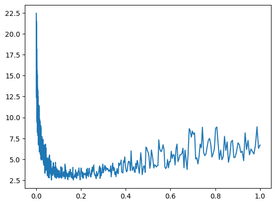
Often, you are going to find that your plot looks something like this, in the beginning you have very low learning rate so barely anything happened, then we got to a nice spot just before the 0.2 ish and as we increased the learning rate enough we got more unstable. So a good learning rate turns out to be somewhere in between 0.0 and 0.2, maybe 0.1.
Actually, it might be better to not track the learning rate but rather the exponent so that would be lre[i] is maybe what we will log, so let me reset this and re run everything and we get this plot:
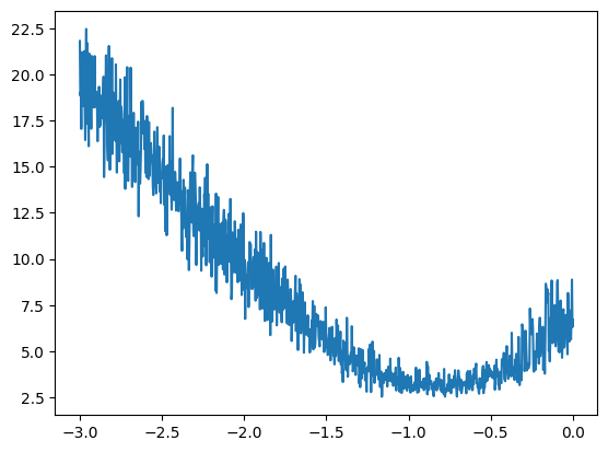
So now at the x axis we have the exponent of the learning rate, we can see that the exponent of the learning rate that would be good to use is roughly in the valley there, somewhere around -1 as the exponent of the learning rate is a pretty good setting and 10 to the power of -1 is 0.1, so 0.1 was actually a fairly good learning rate. This is roughly how you would determine a good learning rate.
So no we can take out the tracking of those and just set the lr to be 10**-1 or just 0.1. Now we have some confidence that this is actually a fairly good learning rate. Now we can crank up the iterations and run for a pretty long time using this learning rate.
After letting that run five times I achieve a loss of the entire dataset of 2.3530 and now I'm going to do learning rate decay, so I'll take the learning rate, lower it by 10x because we are potentially at the late stages of training and we may want to go a bit slower. By the way, the bigram learning rate that we achieved in part 1 was about 2.45, so we have already surpassed the bigram model.
After a single run with the learning rate decay I achieve a loss of 2.2911, of course this is janky and not exactly how you would train it in production but this is roughly what you are going through. You first find a decent learning rate using the approach that I showed you, then start with that learning rate and train for a while and then at the end people like to do a learning rate decay where you decay the learning rate by say a factor of 10 and you do a few more steps and then you get a trained network, roughly speaking.
So after a couple more runs I am now at 2.2874 and dramatically improved from the bigram language model using this simple neural net as described from the paper using our 3481 parameters.
Now, there is something we have to be careful with, I said that we have a better model because we are achieving a lower loss, 2.2874 is lower than 2.45 with the bigram model previously. Now that's not exactly true, the reason is that this is a very small model, only 3481 parameters, but they can get bigger and bigger if that number goes up, there can be millions of parameters. Essentially, as the capacity of the neural network grows it becomes more and more capable of overfitting your training set, this means that the loss on the training set will become very very low, as low as 0, but all that the model is doing is memorising the training set verbatim.
So if you take that model and it looks like its working really well but you try to sample from it, you will basically only get examples exactly as they are in the training set, you won't get any new data. In addition to that, if you try to evaluate the loss from some withheld names, not in the training set, you will see that the loss on those will be very high. So basically it's not a good model.
The standard in this field is to split up your data into 3 splits, the training split, the dev/validation split and the test split. Typically, it's 80%, 10%, 10% respectively. The training split is used to optimise the parameters of the model, just like we just did using gradient descent. The dev/validation split is used for development over all the hyperparameters of your model, so for example the size of our hidden layer, the size of the embedding, currently I'm using 100 and 2 respectively but we could use other numbers, could also be the strength of the regularisation, which I'm currently not using. There's lots of different hyperparameters and settings that go into defining a neural net and you can try many different variations of them and see whichever one works best on your validation split.
So the first split is used to train the parameters, the second split is used to train the hyperparameters and the test split is used to evaluate the performance of the model at the very end. So we are only evaluating the loss on the test split very few times because every single time you evaluate your test loss and you learn something from it, you are basically starting to also train on the test split, so then you would overfit to it as well.
So let's also split up our data into train, dev and test splits, then we are going to train on training split and only evaluate on test very sparingly.
So let's go back to where we built the dataset and put them into tensors. I'm going to convert that part into a function now:
# build the dataset

def build_dataset(words):
    block_size = 3
    X, Y = [], []
    for w in words:

        context = [0] * block_size
        for ch in w + '.':
            ix = stoi[ch]
            X.append(context)
            Y.append(ix)
            context = context[1:] + [ix]

    X = torch.tensor(X)
    Y = torch.tensor(Y)
    print(X.shape, Y.shape)
    return X, Y

import random
random.seed(42)
random.shuffle(words)
n1 = int(0.8*len(words))
n2 = int(0.9*len(words))

Xtr, Ytr = build_dataset(words[:n1])
Xdev, Ydev = build_dataset(words[n1:n2])
Xte, Yte = build_dataset(words[n2:])
This function takes in some list of words and build the arrays X and Y for those words only, after that I randomly shuffly up all the words, I then set n1 to be at the 80% mark of all the words and n2 at the 90% mark. For example, if our list of words is 32,033 words long, then our n1 is 25,626 and n2 is 28,829.
I then call that build_dataset function to first build the training set by indexing the words up to n1, so that will give us 25k training words. Then I'm going to have n2 - n1 = 3203 validation examples and then len(words) - n2 = 3204 examples in the test dataset. After running that:
torch.Size([182625, 3]) torch.Size([182625])
torch.Size([22655, 3]) torch.Size([22655])
torch.Size([22866, 3]) torch.Size([22866])
Now I have Xs and Ys for all those three splits.
Now, let's go back down to the training code, the dataset that we are now training is the training one Xtr.shape, Ytr.shape, with sizes like this (torch.Size([182625, 3]), torch.Size([182625])), now reset the network and on training we only train using this new dataset, so update theose variables. I'll also update the learning rate to be 0.1 again too and train it for a bit. Now when I evaluate, I'll use the dev dataset:
emb = C[Xdev]
h = torch.tanh(emb.view(-1, 6) @ W1 + b1)
logits = h @ W2 + b2
loss = F.cross_entropy(logits, Ydev)
Ok, after training the model a couple times, and then a couple more times with the decayed learning rate I'm getting 2.2679 loss on the dev dataset. So when the neural network was training it hasn't seen those dev examples, it hasn't optimised on them and yet when we evaluate the loss on this dev dataset we actually get a pretty decent loss. If I look at what the loss is on the training set: 2.2671 I see that they are about equal, so we are not overfitting, this model is not powerful enough to be just purely memorising the data and so far we are actually underfitting because these two numbers are roughly equal. This typically means is that our network is very tiny, we expect to make performance improvements by scaling up the size of this neural net, so let's do that now!
The easiest way to increase the size of a neural net is to come to the hidden layer, which currently has 100 neurons, and let's just bump this up to 300 neurons, this would mean we need to update our biases to also be 300 and the inputs into the final layer to be 300:
g = torch.Generator().manual_seed(2147483647)
C = torch.randn((27, 2), generator=g)
W1 = torch.randn((6, 300), generator=g)
b1 = torch.randn((300), generator=g)
W2 = torch.randn((300, 27), generator=g)
b2 = torch.randn((27), generator=g)
parameters = [C, W1, b1, W2, b2]
Let's now initialise the NN, we now have 10281 parameters. Now in the training code, let's track stats again but also let's keep track of the steps this time and let's run this to optimise the neural net:
lri = []
lossi = []
stepi = []

for i in range(30000):

    # minibatch construc
    ix = torch.randint(0, Xtr.shape[0], (32, ), generator=g)

    # forward pass
    emb = C[Xtr[ix]]
    h = torch.tanh(emb.view(-1, 6) @ W1 + b1)
    logits = h @ W2 + b2
    loss = F.cross_entropy(logits, Ytr[ix])


    for p in parameters:
        p.grad = None
    loss.backward()


    lr = 0.1
    for p in parameters:
        p.data += -lr * p.grad

    # track stats
    stepi.append(i)
    lossi.append(loss.item())
Once, this is done I'm going to plot the steps against the loss with plt.plot(stepi, lossi) which gives me this:
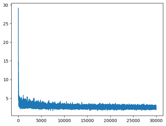
This is the loss function and how it's being optimised, there is quite a bit of thickness to the line and that's because we are optimising over these mini batches and they create some noise. After that first run, we are at 2.4961 loss in the dev set, that's probably because we made it bigger and so it will take longer for this neural net to converge, so let's continue training.
One possibility is also that the batch size is so low that we have way too much noise in the training, so we may want to increase the batch size so that we have a bit more correct gradient and we are not thrashing too much and we can optimise more properly.
After some more training it seems like it's not lowering the loss as much as I expected. One other concern is that even though we have made the hidden layer much bigger it could be that the bottleneck of the network right now are the embeddings that are 2 dimensional, it could be that we are cramming way too much characters into just 2 dimensions and the neural net is not able to really use that space effectively.
One more thing that I want to do is to visualise the embedding vectors for these characters before we scale up the embedding size from 2, because we'd like to make this bottleneck potentially go away and once I make this greater than 2 we won't be able to visualise them. After training somre more and running the evaluation on the training and the dev sets I got these numbers respectively: 2.2070 and 2.2205. This tells me that we are not improving much more and so maybe the bottleneck now is the character embedding size which is currently 2.
plt.figure(figsize=(8, 8))
plt.scatter(C[:, 0].data, C[:, 1].data, s=200)
for i in range(C.shape[0]):
    plt.text(C[i,0].item(), C[i,1].item(), itos[i], ha='center', va='center', color='white')
plt.grid('minor')
So here is the code that creates the figure and then visualise the embeddings that were trained by the neural net on these characters. Right now the embedding size is just 2, so we can visualise all the characters with the x and the y coordinates as the two embedding locations for each of these characters:
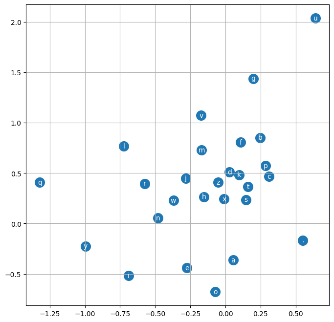
So here what we see is actually kind of interesting, the network has basically learned to separate out the characters and cluster them a little bit, so for example you see how the vowels are all clustered up in the bottom left, this tells me that the neural net treats these as very similar, almost like interchangeable. A point that is really far away is like q, q is treated as an exception, it has a special embedding vector, similarly "." goes the same way, its all the way at the bottom. So it's kind of interesting that there is a little bit of structure after the training and its definitely not random and they kind of make sense.
Ok, now I will scale up the embedding size and won't be able to visualise it directly but I expect that because we are underfitting and we already made the hidden layer much bigger which did not sufficiently improve the loss we're thinking that the constraint to better performance right now could be our embedding vectors. So let's make them bigger.
So if I go up to where we initialise our parameters and we instead of having 2 dimensional embedding instead make them 10 dimensional, for each word. Then W1 would receive 3x10 so 30 inputs will go into the hidden layer, let's also bring the hidden layer down from 300 to 200 neurons:
g = torch.Generator().manual_seed(2147483647)
C = torch.randn((27, 10), generator=g)
W1 = torch.randn((30, 200), generator=g)
b1 = torch.randn((200), generator=g)
W2 = torch.randn((200, 27), generator=g)
b2 = torch.randn((27), generator=g)
parameters = [C, W1, b1, W2, b2]
So now the total number of parameters is: 11897, slightly larger. Then set the learning rate back to 0.1, also we are currently hard coding 6 in the training code, of course in production we don't want to hard code magic numbers but for now it's fine, instead of 6 it should now also be 30, and I'm going to run this for 50,000 iterations.
After running that and logging the log loss against the steps I see this graph:
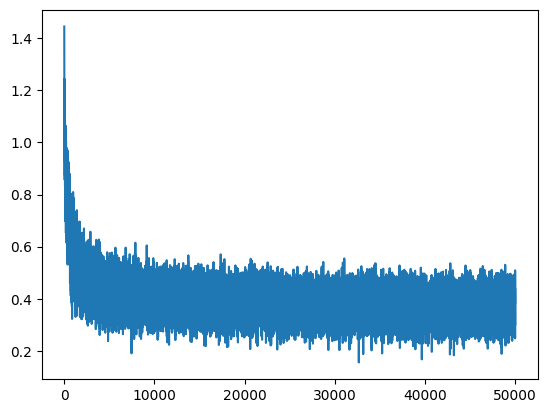
The loss on the training set is 2.3366 and te dev set is 2.3590, so far so good. Let's now decrease the learning rate by a factor of 10. After training that I get 2.1780 on trainig set and 2.2053 on dev set.
You see now how the training and the dev set are starting to slowly move apart now so maybe we are getting the sense that the neural net or that the number of parameters are large enough that we are slowly starting to overfit.
After running it 2 more times I got training loss of 2.1562 and dev loss of 2.1875.
Ok, there's many ways to go from here, we can continue tuning the optimisation, continue playing with the hyperparameters of the neural net or increase the number of characters that we are taking in as an input, so instead of just 3, could take in more and that could further improve the loss.
So now, to sample from the model:
# sample from the 'neural net' model
g = torch.Generator().manual_seed(2147483647)

for _ in range(20):
    out = []
    context = [0] * block_size
    while True:
        emb = C[torch.tensor([context])]
        h = torch.tanh(emb.view(1, -1) @ W1 + b1)
        logits = h @ W2 + b2
        probs = F.softmax(logits, dim=-1)
        ix = torch.multinomial(probs, num_samples=1, generator=g).item()
        context = context[1:] + [ix]
        out.append(itos[ix])
        if ix == 0:
            break

    print(''.join(out))
So we are going to generate 20 samples and at first we begin with all dots and then until we generate another dot (0th character) we embed the current context.
ceri.
kaemonurailah.
tyhamellistana.
nylandr.
kaida.
samiyah.
javar.
gotti.
moziellah.
jacoteda.
kaley.
maside.
enkavion.
ryslam.
huniden.
tahlasu.
jade.
breenley.
alaisa.
jana.
Now these are much more name-like when compared to the results from sequentia part 1, "jana", "alaisa", "kaley", we are definitely makeing progress but we can still improve on this model quite a lot, so onto part 3.
Thanks for reading :)