The goal of sequentia is to simply make more of the things that you give it. For example, names.txt is an example dataset, it is just a large dataset of names, to be specific 32 thousand names. If we train sequentia on this dataset it should learn to make more of things like this, in this particular case, more things that sound name like but are actually unique names. Here are some example generations from sequentia:
dontell
khylum
camatena
aeriline
najlah
sherrith
ryel
irmi
taislee
mortaz
akarli
maxfelynn
biolett
zendy
laisa
halliliana
goralynn
brodynn
romima
chiyomin
loghlyn
melichae
mahmed
irot
helicha
besdy
ebokun
lucianno
These all sound name like. Under the hood, sequentia is a character level language model, so it is treating every single line in names.txt as an example and within each example it is treating them as sequences of individual characters. That is the level on which sequentia is built on, hence the name (latin for sequence).
Sequentia implements a large number of character level language model:
- Bigram
- Bag of words
- MLP
- RNN
- GRU
- Transformer
In fact the transformer that I will build will be basically the equivalent transformer to GPT 2, so it's kind of a big deal as it is a modern network.
So like before with zdravkograd, I will start with a completely blank jupyter notebook.
First let's load up the dataset (names.txt)
words = open('names.txt', 'r').read().splitlines()So lets open up the file in read mode and read in everything into a massive string, and because it's a massive string initially we need to split it into the individual words as a python list of strings.
So if we look at the first 10 words with words[:10] we see this list:
['emma',
 'olivia',
 'ava',
 'isabella',
 'sophia',
 'charlotte',
 'mia',
 'amelia',
 'harper',
 'evelyn']
Let's also quickly take a look at the total number of words with len(wods) which comes out to be 32033.
Also let's see what is for example the shortest word with this code:
min(len(word) for word in words)which comes out to be 2.
And the longest word with:
max(len(word) for word in words)which is 15.
Ok, now, as I mentioned, a character level language model is predicting the next character in a sequence given already some concrete sequence of characters before it.
So if you think about it, isabella for example is like quite a few examples packed into that single word. What is then, the existance of the word isabella in this dataset really telling us? It tells us that the character i is a likely character to come first in a sequence of a name. The character s is likely to come after i, the character a is likely to come after 'is', the character b is likely to come after 'isa' and so on, until finally the character a is likely to come after 'isabell'. But there is actually one more example actually packed in here and that is that after the characters 'isabella' the word is likely to end. So that is one more sort of explicit piece of information that we have here. And so there is actually a lot packed into a single individual word in terms of the statistical structure of what's likely to follow in these character sequences. And then of course we don't have a single word but 32 thousand of them, so there is a lot of structure here to model.
Now first what I will do is build a Bigram language model. Now in a bigram language model, we are always working with just 2 characters at a time, so we are only looking at one character that we have given, and we are trying to predict the next character in the sequence.
So it's a very simple and weak language model, but it's a great place to start.
Let's begin by looking at these bigrams in our dataset and see what they look like.
for w in words[:1]:
    for ch1, ch2 in zip(w, w[1:]):
        print(ch1, ch2)
So for w in words, each w here is an individual word expressed as a string, we want iterate through this word two characters at a time essentially sliding through the word. Above is a very neat way to do this in python, also let's not do this for all the words but just the first word for now, and we get:
e m
m m
m a
The reason this works is because w is the string emma, w[1:] is the string mma, and zip takes two iterators and it pairs them up and creates an iterator over the tuples of their consecutive entries. If any one of these lists is shorter than the other then it will just halt and return. So these are the consecutive elements in the first word, now we have to be careful because we actually have more information here than just these three examples. As we can see, e is likely to come first and we know that a in this case is likely to come last.
chs = ['<S>'] + list(w) + ['<E>']So what we do is we create a special array or characters and we will hallucinate a special start token, for example something like <S>, then we add on the characters from the word as well as another special end character <E>. We now run the previous code with this making sure we use the new list rather than w:
for w in words[:1]:
    chs = ['<S>'] + list(w) + ['<E>']
    for ch1, ch2 in zip(chs, chs[1:]):
        print(ch1, ch2)
and we get this
<S> e
e m
m m
m a
a <E>
Now we can see two extra bigrams added on with the new special charcters.
In order to learn the statistics about which character are likely to follow other character, the simplest way in the bigram language model is to simply do it by counting. So we just need to count how often any one of these combinations occurs in the training set. So we will need some kind of a dictionary that will maintain some count for every one of these bigrams. So let's create some dictionary b = {}. This will map these bigrams: bigram = (ch1, ch2) so bigram is a tuple of character 1 and character 2. Then b at bigram will be b.get(bigram) which is the same as b[bigram], but in the case where bigram is not in the dictionary we will by default return 0, and then + 1. So this code (below) will basically add up these bigrams and count how often they occur. (bumping up to first 3 words rather than just the first)
b = {}
for w in words[:3]:
    chs = ['<S>'] + list(w) + ['<E>']
    for ch1, ch2 in zip(chs, chs[1:]):
        bigram = (ch1, ch2)
        b[bigram] = b.get(bigram, 0) + 1
        print(b)
Now printing our dictionary b we see this:
{('<S>', 'e'): 1,
 ('e', 'm'): 1,
 ('m', 'm'): 1,
 ('m', 'a'): 1,
 ('a', '<E>'): 3,
 ('<S>', 'o'): 1,
 ('o', 'l'): 1,
 ('l', 'i'): 1,
 ('i', 'v'): 1,
 ('v', 'i'): 1,
 ('i', 'a'): 1,
 ('<S>', 'a'): 1,
 ('a', 'v'): 1,
 ('v', 'a'): 1}
Here we can see that many bigrams occur just a single time, but also you can see that a was an ending character 3 times, which is true. Now let's do it for all the characters!
b = {}
for w in words:
    chs = ['<S>'] + list(w) + ['<E>']
    for ch1, ch2 in zip(chs, chs[1:]):
        bigram = (ch1, ch2)
        b[bigram] = b.get(bigram, 0) + 1
Then if we inspect b we see this:
{('<S>', 'e'): 1531,
 ('e', 'm'): 769,
 ('m', 'm'): 168,
 ('m', 'a'): 2590,
 ('a', '<E>'): 6640,
 ('<S>', 'o'): 394,
 ('o', 'l'): 619,
 ('l', 'i'): 2480,
 ('i', 'v'): 269,
 ('v', 'i'): 911,
 ('i', 'a'): 2445,
 ('<S>', 'a'): 4410,
 ('a', 'v'): 834,
 ('v', 'a'): 642,
 ('<S>', 'i'): 591,
 ('i', 's'): 1316,
 ('s', 'a'): 1201,
 ('a', 'b'): 541,
 ('b', 'e'): 655,
 ('e', 'l'): 3248,
 ('l', 'l'): 1345,
 ('l', 'a'): 2623,
 ('<S>', 's'): 2055,
 ('s', 'o'): 531,
 ('o', 'p'): 95,
...
 ('z', 'd'): 2,
 ('x', 'm'): 1,
 ('w', 'g'): 1,
 ('t', 'b'): 1,
 ('z', 'x'): 1}
So these are the counts for all the individual bigrams! We can now look some of the common ones and least common ones, which is kinda gross in python but the way to do this is we use b.items(), this returns the tuples of keys and values where the keys are the character bigrams and the values are the counts. So then we take the sorted() of that but by default sort is on the first item of a tuple but we want to sort by the counts which are the second element of our tuples. So we do this:
sorted(b.items(), key=lambda kv: kv[1])So we use the key which is a lambda function that takes the key value kv and returns the key value at 1, not at 0 but at 1, which is the count.
[(('q', 'r'), 1),
 (('d', 'z'), 1),
 (('p', 'j'), 1),
 (('q', 'l'), 1),
 (('p', 'f'), 1),
 (('q', 'e'), 1),
 (('b', 'c'), 1),
 (('c', 'd'), 1),
 (('m', 'f'), 1),
 (('p', 'n'), 1),
 (('w', 'b'), 1),
 (('p', 'c'), 1),
 (('h', 'p'), 1),
 (('f', 'h'), 1),
 (('b', 'j'), 1),
 (('f', 'g'), 1),
 (('z', 'g'), 1),
 (('c', 'p'), 1),
 (('p', 'k'), 1),
 (('p', 'm'), 1),
 (('x', 'n'), 1),
 (('s', 'q'), 1),
 (('k', 'f'), 1),
 (('m', 'k'), 1),
 (('x', 'h'), 1),
...
 (('e', '<E>'), 3983),
 (('<S>', 'a'), 4410),
 (('a', 'n'), 5438),
 (('a', '<E>'), 6640),
 (('n', '<E>'), 6763)]
And as you can see these are the least common bigrams and to get the most common ones we can do the same thing but in reverse order using this code:
sorted(b.items(), key=lambda kv: kv[1], reverse=True)This returns the reverse order:
[(('n', '<E>'), 6763),
 (('a', '<E>'), 6640),
 (('a', 'n'), 5438),
 (('<S>', 'a'), 4410),
 (('e', '<E>'), 3983),
 (('a', 'r'), 3264),
 (('e', 'l'), 3248),
 (('r', 'i'), 3033),
 (('n', 'a'), 2977),
 (('<S>', 'k'), 2963),
 (('l', 'e'), 2921),
 (('e', 'n'), 2675),
 (('l', 'a'), 2623),
 (('m', 'a'), 2590),
 (('<S>', 'm'), 2538),
 (('a', 'l'), 2528),
 (('i', '<E>'), 2489),
 (('l', 'i'), 2480),
 (('i', 'a'), 2445),
 (('<S>', 'j'), 2422),
 (('o', 'n'), 2411),
 (('h', '<E>'), 2409),
 (('r', 'a'), 2356),
 (('a', 'h'), 2332),
 (('h', 'a'), 2244),
...
 (('j', 'b'), 1),
 (('x', 'm'), 1),
 (('w', 'g'), 1),
 (('t', 'b'), 1),
 (('z', 'x'), 1)]
So n was very often an ending character and so on. These are the individual counts that we can achieve over the entire dataset.
It's actually going to be much more convenient to keep this information in a 2 dimensional array instead of a python dictionary. We will have the rows be the first character and the columns are going to be the second character and each entry in this 2d array will tell us how often the second character follows the first character in the dataset. To do this I will use PyTorch and its tensors, these tensors allow us to create multi dimentional arrays and manipulate them very efficiently.
So let's import PyTorch with import torch, now we will create an array of zeros, let's do this for an example.
a = torch.zeros((3, 5))and printing a we see this:
tensor([[0., 0., 0., 0., 0.],
        [0., 0., 0., 0., 0.],
        [0., 0., 0., 0., 0.]])
and by default we can see that the a.dtype is torch.float32 which tells us that we have single precision floating point numbers. Because we are representing a count let's use the dtype of torch.int32, so these are 32 bit integers.
tensor([[0, 0, 0, 0, 0],
        [0, 0, 0, 0, 0],
        [0, 0, 0, 0, 0]], dtype=torch.int32)
Now of course, the array that we are interested in is bigger, for our purposes we have 26 letters of the alphabet and then we also have 2 special characters <S> and <E> so we will need a 28 by 28 array.
N = torch.zeros((28, 28), dtype=torch.int32)Ok now we will go back and use that code from above but change it to use our new N array, only issue is that we used strings in the previous code and now we need to be indexing into this new 2d array which uses integers, we will need some kind of a lookup table from characters to integers.
The way we are going to do this is by taking all the words, concatenate all of it into a massive string using join() turning the entire dataset into a single string and then pass that into the set() constructor which throws out all the duplicates, essentially just giving us all the lower case characters used in our dataset.
set(''.join(words))which gives us this:
{'a',
 'b',
 'c',
 'd',
 'e',
 'f',
 'g',
 'h',
 'i',
 'j',
 'k',
 'l',
 'm',
 'n',
 'o',
 'p',
 'q',
 'r',
 's',
 't',
 'u',
 'v',
 'w',
 'x',
 'y',
 'z'}
and with len(set(''.join(words))) we can see that there is in fact 26 of them. Now we don't want a set we want a list: list(set(''.join(words))), we also don't want a list sorted in some arbitrary way we want it to be sorted from a to z: sorted(list(set(''.join(words)))). Good now we have our list or characters.
Now we need that look-up table, let's call it stoi (string to integer), and this will be an s to i mapping for i:s in enumerate of these chracters. Enumerate gives us this iterator over the integer index and the actual element of the list, and then we are mapping the character to the integer.
chars = sorted(list(set(''.join(words))))
stoi = {s:i for i,s in enumerate(chars)}
So now, stoi:
{'a': 0,
 'b': 1,
 'c': 2,
 'd': 3,
 'e': 4,
 'f': 5,
 'g': 6,
 'h': 7,
 'i': 8,
 'j': 9,
 'k': 10,
 'l': 11,
 'm': 12,
 'n': 13,
 'o': 14,
 'p': 15,
 'q': 16,
 'r': 17,
 's': 18,
 't': 19,
 'u': 20,
 'v': 21,
 'w': 22,
 'x': 23,
 'y': 24,
 'z': 25}
Finally, we have to also specifically set those last two special chars with stoi['<S>'] = 26 and stoi['<E>'] = 27. Lookup table complete.
Now we can go back to our previous code and we can map both character 1 and character 2 to their integers
for w in words:
    chs = ['<S>'] + list(w) + ['<E>']
    for ch1, ch2 in zip(chs, chs[1:]):
        ix1 = stoi[ch1]
        ix2 = stoi[ch2]
        N[ix1, ix2] += 1
So now using the code above we can map both characters 1 and 2 to their integers, as well as using the 2d array indexing and add one to that specific mapping. Now if we print N we can see the 2d array:
tensor([[ 1112,  1082,   940,  2084,  1384,   268,   336,  4664,  3300,   350,
          1136,  5056,  3268, 10876,   126,   164,   120,  6528,  2236,  1374,
           762,  1668,   322,   364,  4100,   870,     0, 13280],
        [  642,    76,     2,   130,  1310,     0,     0,    82,   434,     2,
             0,   206,     0,     8,   210,     0,     0,  1684,    16,     4,
            90,     0,     0,     0,   166,     0,     0,   228],
        [ 1630,     0,    84,     2,  1102,     0,     4,  1328,   542,     6,
           632,   232,     0,     0,   760,     2,    22,   152,    10,    70,
            70,     0,     0,     6,   208,     8,     0,   194],
        [ 2606,     2,     6,   298,  2566,    10,    50,   236,  1348,    18,
             6,   120,    60,    62,   756,     0,     2,   848,    58,     8,
           184,    34,    46,     0,   634,     2,     0,  1032],
        [ 1358,   242,   306,   768,  2542,   164,   250,   304,  1636,   110,
           356,  6496,  1538,  5350,   538,   166,    28,  3916,  1722,  1160,
           138,   926,   100,   264,  2140,   362,     0,  7966],
        [  484,     0,     0,     0,   246,    88,     2,     2,   320,     0,
             4,    40,     0,     8,   120,     0,     0,   228,    12,    36,
            20,     0,     8,     0,    28,     4,     0,   160],
        [  660,     6,     0,    38,   668,     2,    50,   720,   380,     6,
             0,    64,    12,    54,   166,     0,     0,   402,    60,    62,
           170,     2,    52,     0,    62,     2,     0,   216],
        [ 4488,    16,     4,    48,  1348,     4,     4,     2,  1458,    18,
            58,   370,   234,   276,   574,     2,     2,   408,    62,   142,
           332,    78,    20,     0,   426,    40,     0,  4818],
        [ 4890,   220,  1018,   880,  3306,   202,   856,   190,   164,   152,
...
           156,   752,   614,   268,  1070,  1858,     0,     0],
        [    0,     0,     0,     0,     0,     0,     0,     0,     0,     0,
             0,     0,     0,     0,     0,     0,     0,     0,     0,     0,
             0,     0,     0,     0,     0,     0,     0,     0]],
       dtype=torch.int32)
Only thing is that this looks ugly so let's try to visualise this a bit more nicer. To do that we will use a library called matplotlib which allows us to create figures, so we can do this:
import matplotlib.pyplot as plt
%matplotlib inline
plt.imshow(N)
and with that we can see this figure:
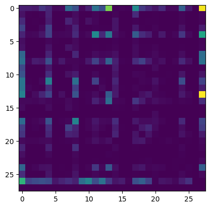
So this is the 28x28 array and its structure but even this is still pretty ugly, so let's create a much nicer visualisation. First thing we need to do is to invert our itos disctionary, itos = {i:s for s,i in stoi.items()}, then we use this code:
import matplotlib.pyplot as plt
%matplotlib inline

plt.figure(figsize=(16,16))
plt.imshow(N, cmap='Blues')
for i in range(28):
    for j in range(28):
        chstr = itos[i] + itos[j]
        plt.text(j, i, chstr, ha="center", va="bottom", color='gray')
        plt.text(j, i, N[i, j].item(), ha="center", va="top", color='gray')
plt.axis('off');
This code gives us this figure:
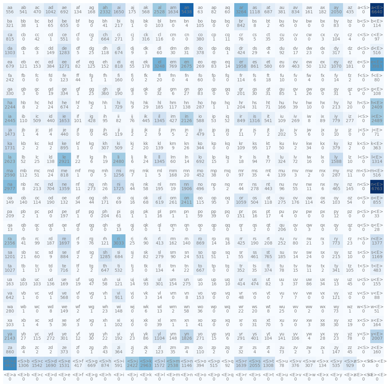
This shows us for example that b follows g 0 times etc. Essentially we show that N array again with imshow, then we map through each one of the little squares and we create a character string, which is the inverse mapping (itos) of the integer i and the integer j, so our bigram in a charcter representation again. That bigram gets plotted on the square and then under it we also plot how many times it occurs.
If you look at this carefully, you will notice that we are not actually being very clever, the bottom row is an entire row of completely zeros and that is because the end character is never possibly going to be the first character of a bigram. Similarly, we have an entire column of zeros where the special start character comes after some initial character, which again is impossible. So we are basically wasting space, on top of that the special character are getting very crowded, this was done initially as its a convention in natural language processing to use these angle brackets to denote special tokens but from now we will use something else.
From now on, we will not have two special tokens but only one actually, so we will have a 2d array that will be 27x27 instead. Our singular special character will simply be a dot. Also, instead of putting that special character on the end we will actually place it in position 0 and then shift all our other character one space up, this looks more pleasing. Now modifying our other code to fit these changes and plotting our figure we now see this:
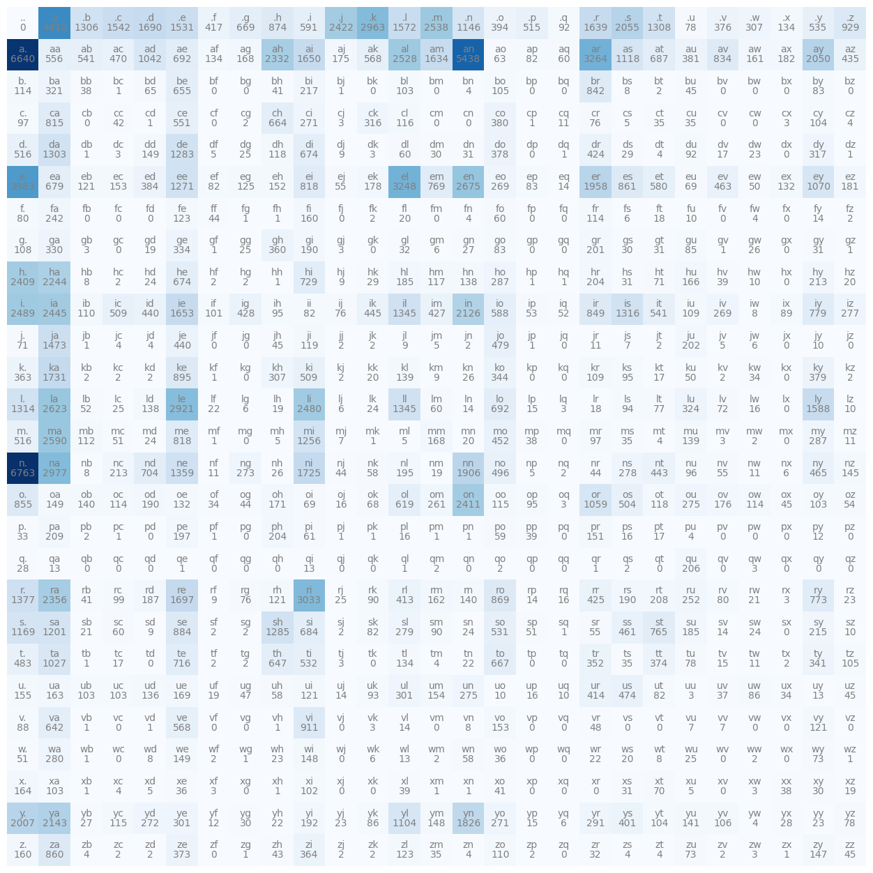
We now see that .. never happened because we don't have empty words, that first row shows us the count of all the first letters etc.
This array now has all the information necessary for us to sample from this bigram character level language model. Roughly speaking we are just going to start following these probabilities and these counts and just start sampling frmo the model.
In the beginning of course we start with the dot, so to sample the first character of the name we are looking at this first row. So it we take our arry and grab that first row by indexing at 0 N[0, :], and using that colon we grab the rest of that row which looks like this:
tensor([   0, 4410, 1306, 1542, 1690, 1531,  417,  669,  874,  591, 2422, 2963,
        1572, 2538, 1146,  394,  515,   92, 1639, 2055, 1308,   78,  376,  307,
         134,  535,  929], dtype=torch.int32)
We can also actually just use N[0], that is equivalent. Now let's sample from this. Since these are the raw counts are actually have to convert these into probabilities. Let's create a probability vector, we will take N[0] and convert that to float, this is because we are about to normalise these counts.
p = N[0].float()
p = p / p.sum()
p
We divide by the sum and now we have this:
tensor([0.0000, 0.1377, 0.0408, 0.0481, 0.0528, 0.0478, 0.0130, 0.0209, 0.0273,
        0.0184, 0.0756, 0.0925, 0.0491, 0.0792, 0.0358, 0.0123, 0.0161, 0.0029,
        0.0512, 0.0642, 0.0408, 0.0024, 0.0117, 0.0096, 0.0042, 0.0167, 0.0290])
This shows us the probability for any single character to be the first character of a word. To now sample from this distribution we will use torch.multinomial, this samples from the multinomial probability distribution, which is a complicated way of saying: you give me probabilities and I'll give you integers which are sampled according to the given probabiilty distribution. To make everything deterministic we will use a generator object in PyTorch, this is so when this is run on a different computer it will give the exact same results that I get in my jupyter notebook.
g = torch.Generator().manual_seed(2147483647)
p = torch.rand(3, generator=g)
p = p / p.sum()
So we first seed a generator that gives us an object we will call g, then we pass that object g to a function that creates random numbers, 3 of them in our case. We also normalise this and we get a nice probability distribution of 3 elements: tensor([0.6064, 0.3033, 0.0903]). And then we can use torch.multinomial to draw samples from it.
torch.multinomial(p, num_samples=20, replacement=True, generator=g)So it takes the torch tensor of probability distributions, then we ask for a number of samples, 20 in this case, we also set replacement to true because by default its false in pytorch, and finally we also pass in the generator to make sure we always get deterministic results. So if we run this we get these samples:
tensor([1, 1, 2, 0, 0, 2, 1, 1, 0, 0, 0, 1, 1, 0, 0, 1, 1, 0, 0, 1])Now you will notice that the probability in the first tensor is 60%, so in these 20 samples we should expect 0 to occur 60% of the time and so on.
For us, we are interested in the first row of N, we have our p and we use that as the probability distribution and sample from it the same way:
g = torch.Generator().manual_seed(2147483647)
ix = torch.multinomial(p, num_samples=1, replacement=True, generator=g).item()
ix
we output the index ix at the end and we see 3, and of course we can map to the character using itos[ix] to see the exact character which turns out to be 'c'. So that will be the first character of our word and now we can continue to sample more characters. We need to find the row that starts with our character. But instead of doing this manually let's write out the loop that will do this for us as we know have a sense of how this is going to go with that first example.
g = torch.Generator().manual_seed(2147483647)

ix = 0
while True:
    p = N[ix].float()
    p = p / p.sum()
    ix = torch.multinomial(p, num_samples=1, replacement=True, generator=g).item()
    print(itos[ix])
    if ix == 0:
        break
We always begin at index 0, that is the start token, then while true we need to grab the row of the index that we are currently on, get the probability distribution for that row and sample from it, if its the ending character (.) then we break so we don't have an infinite loop and that's it.
g = torch.Generator().manual_seed(2147483647)

for i in range(10):
    out = []
    ix = 0
    while True:
        p = N[ix].float()
        p = p / p.sum()
        ix = torch.multinomial(p, num_samples=1, replacement=True, generator=g).item()
        out.append(itos[ix])
        if ix == 0:
            break
    print(''.join(out))
Now let's do this a few times too so let's create an out list, now we will always get the same result because of the generator but let's do this 10 times and see what we get.
cexze.
momasurailezitynn.
konimittain.
llayn.
ka.
da.
staiyaubrtthrigotai.
moliellavo.
ke.
teda.
lol, so these don't look right, but they actually are, it's just that bigram language models are just absolutely terrible. One way we can check to kind of convince ourselves more that this is actually working is instead of using our distributions from the data let's just use this p = torch.ones(27) / 27.0. This is the uniform distribution which makes everything equally likely, and if we sample from that we see these results:
cexzm.
zoglkurkicqzktyhwmvmzimjttainrlkfukzkktda.
sfcxvpubjtbhrmgotzx.
iczixqctvujkwptedogkkjemkmmsidguenkbvgynywftbspmhwcivgbvtahlvsu.
dsdxxblnwglhpyiw.
igwnjwrpfdwipkwzkm.
desu.
firmt.
gbiksjbquabsvoth.
kuysxqevhcmrbxmcwyhrrjenvxmvpfkmwmghfvjzxobomysox.
This is what we get from a model that is completely untrained where everything is equally likely so it's obviously trash and comparing it to the trained model results from above we can see that its results are actually kind of name like.
Next, I would like to fix an inefficiency in our code, specifically in these two lines
p = N[ix].float()
p = p / p.sum()
We are always fetching a row of N from the counts matrix and we are always doing the same thing: converting to float and dividing, and we are doing this every single iteration of this loop, so we just keep re normalising these rows over and over again which is extremely inefficient and wasteful. So instead, let's prepare a matrix P that will just have the probabilities in it. So it will be the same matrix as above but every single row will have a row of probabilities that is normalised to 1. That way in our code we can just use P[ix] instead of those two lines.
P = N.float()
P = P / P.sum(1, keepdim=True)
So here we start by converting our count matrix N to floating point numbers, which we need because we're about to do division and we want decimal probabilities instead of whole numbers. Then on the next line we normalise each row of the matrix, where P.sum(1, keepdim=True) sums across each row (the 1 means we're summing along dimension 1, which is the columns), and keepdim=True ensures the result keeps the same number of dimensions so we can broadcast the division properly. When we divide each row by its sum, every row now represents a proper probability distribution where all the values add up to 1, which is exactly what we need for sampling with torch.multinomial. Now instead of recalculating these probabilities every single time we sample a character, we can just grab the precomputed row P[ix] and use it directly, which is much more efficient.
Now again, we got to be careful, is it possible to take a 27x27 array and divide it by a 27x1 array, whether or not we can do this operation is determined by whats called broadcasting rules. We have these special conditions (see link) for broadcasting on whether or not these two arrays can be combined in a binary operation like division.
The first condition is that each tensor must have at least one dimension which is true in our case and then, when iterating over the dimension sizes, starting at the trailing dimension, the dimension sizes must either be equal, one of them is 1 or one of them does not exist. So we align the dimensions up like this
27, 27
27, 1
So starting from the right we compare, in the first case we have 27 and 1, which is good because one of them is a 1, so it's fine, and in the second one, we have 27 and 27, which are both equal and so that is fine as well. So all the dimensions are fine and so this operation is broadcastable. And what happens when we do this division between a 27x27 and a 27x1 array? It stretches out the 1 dimension, copying it over to match 27. And we can check if it worked correctly by taking the first row for example and checking if its sum is 1, P[0].sum() = tensor(1.). Perfect it's now normalised, and if we re run our previous code to get the "names" we should get the exact same result, and we do!
Now what would happen if we didn't use keepdim=True? Well, P.sum(1) would produce a tensor of shape (27,) instead of (27, 1), which contains the sum of each row. When we try to divide our (27, 27) tensor by this (27,) tensor, PyTorch's broadcasting aligns dimensions from the right, treating the (27,) tensor as (1, 27) rather than (27, 1). This means the division would broadcast that single row of sums across all 27 rows, but it would divide each column by a different row sum value, which is completely wrong. For example, if we had a small 3x3 matrix with row sums [6., 15., 24.], without keepdim=True the division would give us something like [[1/6, 2/15, 3/24], [4/6, 5/15, 6/24], [7/6, 8/15, 9/24]], where each row no longer sums to 1 and the values are meaningless for bigram probabilities. This would completely break our probability matrix, and when we sample from it with torch.multinomial, we'd get garbage sequences that don't reflect the actual bigram statistics from our training data. So keepdim=True is absolutely necessary here to get the correct (27, 1) shape and ensure proper row-wise normalization.
We can also make this even more efficient by using an in-place operation. When we write P = P / P.sum(1, keepdim=True), PyTorch creates a new tensor to hold the result of the division, which means we're temporarily using extra memory. Instead, we can use the in-place division operator /=, which modifies P directly without creating an intermediate tensor. So P /= P.sum(1, keepdim=True) does exactly the same thing but uses less memory, which is especially important when working with larger tensors or when memory is constrained.
Okay, we are now in a pretty good spot, we trained a bigram language model just by counting how frequently any pairing occurs and then normalising so that we get a nice probability distribution. So really the elements of the array P are our parameters of our language model, so we train the model and we know how to sample from the model. Now I would like to have a way to evaluate the quality of this model, somehow summarise the quality of this model into a single number, how good is it at predicting the training set? So in the training set we can evaluate the training loss and this number would tell us the quality of this model.
So let's go back and take this code:
for w in words[:3]:
    chs = ['.'] + list(w) + ['.']
    for ch1, ch2 in zip(chs, chs[1:]):
        ix1 = stoi[ch1]
        ix2 = stoi[ch2]
        print(f'{ch1}{ch2}')
which again gives us these results for the first three words:
.e
em
mm
ma
a.
.o
ol
li
iv
vi
ia
a.
.a
av
va
a.
Now what we would like to do is look at the probability that the model assigns to every single one of these bigrams. We can look at this probability with prob = P[ix1, ix2] and we can add it onto the print statement (print(f'{ch1}{ch2}: {prob:.4f}')) to get this:
.e: 0.0478
em: 0.0377
mm: 0.0253
ma: 0.3899
a.: 0.1960
.o: 0.0123
ol: 0.0780
li: 0.1777
iv: 0.0152
vi: 0.3541
ia: 0.1381
a.: 0.1960
.a: 0.1377
av: 0.0246
va: 0.2495
a.: 0.1960
Just as a measuring stick, we have 27 possible characters/tokens and if everything was equally likely then you would expect these probabilities to be 1/27 which is roughly 4%, so above 4% means that we've learnt something useful from these bigram statistics.
So now how can we summarise these probabilities into a single number that measures the quality of this model. If you take a look at the literature of Maximum Likelihood estimation and statistical modelling and so on, you will see that what's typically used here is something called the likelihood, and that is simply the product of all of these probabilities. Also you will notice that all our numbers are between 0 and 1 and so if you multiply them all you will get a very small number, so for convenience people usually work with the log likelihood instead of the default likelihood. To get the log likelihood you just have to take the log of the likelihood.
log_likelihood = 0.0
for w in words[:3]:
    chs = ['.'] + list(w) + ['.']
    for ch1, ch2 in zip(chs, chs[1:]):
        ix1 = stoi[ch1]
        ix2 = stoi[ch2]
        prob = P[ix1, ix2]
        log_prob = torch.log(prob)
        log_likelihood += log_prob
        print(f'{ch1}{ch2}: {prob:.4f} {log_prob:.4f}')
log_likelihood.e: 0.0478 -3.0408
em: 0.0377 -3.2793
mm: 0.0253 -3.6772
ma: 0.3899 -0.9418
a.: 0.1960 -1.6299
.o: 0.0123 -4.3982
ol: 0.0780 -2.5508
li: 0.1777 -1.7278
iv: 0.0152 -4.1867
vi: 0.3541 -1.0383
ia: 0.1381 -1.9796
a.: 0.1960 -1.6299
.a: 0.1377 -1.9829
av: 0.0246 -3.7045
va: 0.2495 -1.3882
a.: 0.1960 -1.6299
tensor(-38.7856)So log_likelihood is -38.7856, now we have this, but a loss function has the semantics that low is good because we are trying to minimise the loss. So we actually need to invert this, which gives us something called the negative log likelihood.
People also like to normalise the log likelihood by the number of examples, so we get an average log likelihood per example. This makes it easier to compare models trained on different sized datasets. So instead of just summing up all the log probabilities, we divide by the total number of bigrams we've seen. Let's calculate this for the entire training set now:
log_likelihood = 0.0
n = 0
for w in words:
    chs = ['.'] + list(w) + ['.']
    for ch1, ch2 in zip(chs, chs[1:]):
        ix1 = stoi[ch1]
        ix2 = stoi[ch2]
        prob = P[ix1, ix2]
        log_prob = torch.log(prob)
        log_likelihood += log_prob
        n += 1
nll = -log_likelihood
print(f'{n} bigrams, log likelihood: {log_likelihood:.4f}, negative log likelihood: {nll:.4f}')
print(f'average log likelihood per bigram: {log_likelihood/n:.4f}')
So we iterate through all the words, count up all the bigrams with n, accumulate the log likelihood, and then we can calculate the average. The negative log likelihood is just the negative of the log likelihood, which gives us our loss value where lower is better.
Now, there's actually a more efficient way to calculate this. Instead of looping through every word and every bigram, we can use the fact that we already have our count matrix N and probability matrix P. We can calculate the log likelihood directly from these matrices:
log_likelihood = (N * torch.log(P)).sum()
n = N.sum().item()
nll = -log_likelihood
print(f'{n} bigrams, log likelihood: {log_likelihood:.4f}, negative log likelihood: {nll:.4f}')
print(f'average log likelihood per bigram: {log_likelihood/n:.4f}')
Here we're using element-wise multiplication N * torch.log(P), which multiplies each count by its corresponding log probability, and then we sum everything up. This is much faster than looping through all the words, especially for large datasets. The N.sum().item() gives us the total number of bigrams, which we use to calculate the average.
This average negative log likelihood per bigram is a common metric in language modelling, and it tells us how surprised the model is on average by each bigram it sees. Lower values mean the model is less surprised, which means it's doing a better job at predicting the training data.
However, there's a problem with our current approach. What happens if we try to evaluate the model on a word that contains a bigram we've never seen before in the training data? For example, let's say we have a name like "andrejq". If we look at the bigram "jq", this combination might never have appeared in our training set, which means N[stoi['j'], stoi['q']] would be 0. When we calculate the probability P[stoi['j'], stoi['q']], we'd get 0, and when we take torch.log(0), we get negative infinity. This means the log likelihood would be negative infinity, and the loss would be infinity, which completely breaks our evaluation.
This is a fundamental problem in language modelling called the zero probability problem. If our model assigns zero probability to any bigram it hasn't seen, then any sequence containing that bigram will have infinite loss, which isn't very useful. To fix this, we need to use something called smoothing, which ensures that every bigram has at least some small probability, even if we've never seen it before.
The simplest form of smoothing is called additive smoothing, or Laplace smoothing. The idea is very straightforward: we just add 1 to every single count in our matrix N before we normalise it. This way, even bigrams that never appeared in the training data will have a count of 1 instead of 0, which means they'll have a small but non-zero probability. Let's modify our code to do this:
N = torch.zeros((27, 27), dtype=torch.int32)
for w in words:
    chs = ['.'] + list(w) + ['.']
    for ch1, ch2 in zip(chs, chs[1:]):
        ix1 = stoi[ch1]
        ix2 = stoi[ch2]
        N[ix1, ix2] += 1

# Add 1 to all counts for smoothing
N = N + 1

# Now normalise as before
P = N.float()
P /= P.sum(1, keepdim=True)
So we add 1 to every element of N before converting to probabilities. This means that every bigram, even ones we've never seen, will have at least a count of 1, and therefore a non-zero probability. The probabilities will be slightly different now because we're adding 27*27 = 729 extra counts to our matrix, but this ensures that we can evaluate any sequence without running into infinite loss.
Now if we try to evaluate "andrejq", the bigram "jq" will have a small probability instead of zero, and the log likelihood will be a finite number instead of negative infinity. The model will still assign a very low probability to unseen bigrams, which makes sense because they're unlikely, but at least we can compute a meaningful loss value.
Ok, so we have now trained a respectable bigram character level language model, we trained the model by looking at the counts of all the bigrams and normalising the rows to get probability distributions, we used the parameters of this model to sample new words and we also evaluated the quality of this model and it summarised into a single number: the negative log likelihood.
Now, let's take an alternative aproach, we will end up in a very similar position but the aproach will look very different. I will cast the problem of bigram character level language modelling into a neural network framework. It will still be a bigram character level language model, it will still receive a single character as an input, then there is a neural network with some weights and parameters and it's going to output the probability distribution over the next character in the sequence. In addition to that, we are going to be able to evaluate any setting of the parameters of the neural net because we have the loss function (the negative log likelihood). So we will use gradient based optimisation to tune the parameters of this network, because we have the loss function and we are going to minimise it, so we will tune the weights so that the neural net is correctly predicting the probabilities of the next character.
The first thing I want to do is to compile the training set of this neural network:
for w in words:
    chs = ['.'] + list(w) + ['.']
    for ch1, ch2 in zip(chs, chs[1:]):
        ix1 = stoi[ch1]
        ix2 = stoi[ch2]
So here we start with the words, we iterate over all the bigrams, and previously we did the counts but now we are not going to do counts we are just creating a training set. Now this training set will be made of two lists, we have the inputs xs and the targets/labels ys. And our bigrams will denote (x, y) because we will be given the first character and we will try to predict the next one. Both of these lists will also be integers but of course we don't want just simple lists of integers but we will actually create tensors.
# create the training set of all the bigrams
xs, ys = [], []

for w in words:
    chs = ['.'] + list(w) + ['.']
    for ch1, ch2 in zip(chs, chs[1:]):
        ix1 = stoi[ch1]
        ix2 = stoi[ch2]
        xs.append(ix1)
        ys.append(ix2)

xs = torch.tensor(xs)
ys = torch.tensor(ys)
To keep things manageable let's take the first word as an example to talk over which is emma. The xs are:
tensor([ 0, 5, 13, 13, 1])and the ys are
tensor([ 5, 13, 13, 1, 0]and if I also print this print(f'{ch1}{ch2}: {ix1} {ix2}') in the for loop we see can see it more clearly:
.e: 0 5
em: 5 13
mm: 13 13
ma: 13 1
a.: 1 0
So the bigrams of this word are above, this single word has 5 examples for our neural network. These 5 examples are also seen in the xs and ys, for example when the input to the neural network is integer 0, the desired label is integer 5, which corresponds to e. When the input to the neural net is 5 we want its weights to be arranged so that 13 gets a very high probability, and so on.
Small tangent, it is important to be careful with a lot of the APIs with a lot of these frameworks. In the code above I am using torch.tensor with a lower case t and the output looked right but you should be aware that there is actually two ways of constructing a tensor. There is the lower case t tensor and the upper case tensor which is a class that you can construct. Unfortunately, the docs are just not very clear on the difference between the two but there are threads which explain it quite well. Really it comes down to:
In PyTorch torch.Tensor is the main tensor class. So all tensors are just instances of torch.Tensor.
When you call torch.Tensor() you will get an empty tensor without any data.
In contrast torch.tensor is a function which returns a tensor. In the documentation it says:
torch.tensor(data, dtype=None, device=None, requires_grad=False) → TensorConstructs a tensor with data.
This also explains why it is no problem creating an empty tensor instance of torch.Tensor without data by calling:
tensor_without_data = torch.Tensor()But on the other side:
tensor_without_data = torch.tensor()Will lead to an error:
---------------------------------------------------------------------------
TypeError                                 Traceback (most recent call last)
<ipython-input-12-ebc3ceaa76d2> in <module>()
----> 1 torch.tensor()

TypeError: tensor() missing 1 required positional arguments: "data"
Also someone on the thread points out:
torch.tensor infers the dtype automatically, while torch.Tensor returns a torch.FloatTensor. I would recommend to stick to torch.tensor, which also has arguments like dtype, if you would like to change the type.
So I'm pointing out these things so that I know to continue and use these APIs with caution, also to get used to reading a lot of documentation and threads. What we want in our example above is integers and so we are using the lower case t as it can infer that on its own.
Ok now I want to think through how I am going to feed in these examples into a neural network, it's not quite as straight forward as plugging it in because these examples right now are just integers and you can't just plug an integer index into a neural net. If you have read my zdravkograd blog and seen that project you should remember that a neural net has these neurons which act multiplicatively on each other and with the weights, so it doesn't really make sense for them to be integers. So instead a common way of encoding integers is using one hot encoding. In one hot encoding we take an integer like 13 and we create a vector that is all zeros except for the 13th dimension which we turn to a 1, and then that vector can feed into a neural net.
Conveniently, PyTorch actually has a one hot function, it takes a tensor made up of integers (Long is an integer) and it also takes a number of classes, which is how large you want your vector to be.
So let's import it, this is a common way of importing it:
import torch.nn.functional as FAnd then let's do:
xenc = F.one_hot(xs, num_classes=27)We feed in the integers that we want to encode, and we can actually feed in the entire array of xs, we can also specify the num_classes is 27 so it doesn't try to guess it. We can call it xenc for x encoded, and we can see that xenc.shape is torch.Size([5, 27]) (5x27), and we can also visualise it with plt.imshow(xenc) to make it a little bit more clear, and it spits out this:
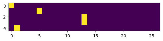
You can see that we have encoded all the 5 examples into vectors, 5 examples, so 5 rows and each row here is now an example into a neural net and you can see that the appropriate bit is turned on as a 1 and everything else is a 0. So that's how we can encode integers into these vectors and then these vectors can feed into neural nets.
One more thing to actually be careful of: let's take a look at xenc's datatype, what would you expect it to be? When we plugging numbers into neural nets we don't want them to be integers, we want them to be floating point numbers that can take on varius values. The dtype here is torch.int64 so 64 bit integer, the reason for that is because the one hot function received a dtype of 64 bit integer so it outputted the same type. In a lot of functions in pytorch you can specify in the function parameters what dtype you would like it to output but one hot does not support that. So instead we will cast this to a float like this xenc = F.one_hot(xs, num_classes=27).float() and then if we examine the dtype of xenc we see it is torch.float32. So now this can feed into a neural net.
Now let's construct our first neuron, this neuron will look at these input vectors and if you remmeber from zdravkograd these neurons perform this very simple function: wx + b, where wx is just a dot product, so we should be able to easily achieve the same thing here.
Let's first define the weights of this neuron, so what are the initial weights at initialisation for this neuron. Let's initialise them with torch.randn, this fills a tensor with random numbers drawn from a normal distribution. So we take size as an input here, and I will use (27, 1). And then let's store that in a variable W and let's see what it looks like:
tensor([[-0.4518],
        [ 0.4064],
        [ 2.4884],
        [-1.0498],
        [-1.0535],
        [ 1.5365],
        [-0.2874],
        [ 0.8388],
        [-0.3718],
        [ 0.0271],
        [ 0.9102],
        [ 1.4895],
        [-0.1133],
        [-2.2174],
        [ 1.8190],
        [ 0.5909],
        [ 2.0329],
        [ 0.7682],
        [ 0.9322],
        [-1.1766],
        [ 0.4649],
        [-1.6743],
        [ 0.9389],
        [-2.0692],
        [ 1.8214],
        [ 0.0315],
        [ 0.9747]])
So W is a column vector of 27 numbers and these weights are then multiplied by the inputs. Now to perform this multiplication we can take xenc and multiply it with W like this xenc @ W the @ is a PyTorch matrix multiplication operator. That gives us this:
tensor([[ 0.9313],
        [-1.4683],
        [-0.5473],
        [-0.5473],
        [-0.3596]])
The output of this operation is 5x1, this is because we multiplied a 5x27 by a 27x1, the 27's will multiply and add. We are essentially seeing the 5 activations of this neuron from these 5 inputs and we evaluated all of them in parallel (pytorch helps with this). But instead of a single neuron I would like 27, I'll tell you why in a bit. But we can just change the code so that its W = torch.randn((27,27)) instead of W = torch.randn((27,1)).
Now we get this:
tensor([[-0.8083, -0.1806,  0.5411, -1.9709, -1.2911,  1.3638, -0.9198, -1.3197,
         -0.9731,  0.9335,  0.2360, -0.4966,  0.0081, -0.5114, -0.6180,  0.6707,
         -0.8448, -0.1883, -0.4675,  1.5044, -1.0876,  0.8690, -0.3955,  1.1926,
          0.0316,  0.2621,  0.3415],
        [ 0.2961,  1.5788, -0.8755,  1.9271, -0.5709, -0.8015,  1.3536,  1.5452,
         -0.5915,  1.0872,  0.6926, -0.2932, -0.3504,  0.7362,  1.2180,  1.3265,
          0.3844, -0.5124,  1.6314,  1.2731,  0.2277, -0.5313, -0.6138, -1.1063,
         -0.8269,  0.2015,  0.6057],
        [-0.0222, -1.4024,  0.4644,  0.2770, -0.7199, -0.8828, -0.3808, -0.2096,
         -0.4294,  0.1786,  1.4026, -0.1493,  0.1361, -0.8037,  1.1314,  0.6296,
          0.0190,  0.3452,  0.0964, -0.6982, -1.0523, -0.6096,  0.0186,  0.7593,
         -0.9675, -0.8365, -1.7953],
        [-0.0222, -1.4024,  0.4644,  0.2770, -0.7199, -0.8828, -0.3808, -0.2096,
         -0.4294,  0.1786,  1.4026, -0.1493,  0.1361, -0.8037,  1.1314,  0.6296,
          0.0190,  0.3452,  0.0964, -0.6982, -1.0523, -0.6096,  0.0186,  0.7593,
         -0.9675, -0.8365, -1.7953],
        [-1.0084, -1.0732,  0.5935,  1.1916,  0.2834,  0.0133, -1.7421,  0.1414,
         -0.2923, -0.0698, -2.5844,  0.8936, -0.2841, -0.9766, -0.6943,  0.8469,
         -0.8529,  0.9908,  0.0906,  0.2939,  0.6630, -0.5760,  0.5404,  1.1129,
         -2.4166, -0.5970,  0.8983]])
So this is a 5x27, and we can confirm this with (xenc @ W).shape which gives out torch.Size([5, 27]), exactly what we expected. But what does every element here tell us? Well, for every 1 of these 27 neurons that we created what is the firing rate on every one of those 5 examples.
For example, the element in (xenc @ W)[3, 13] this position gives me tensor(-0.8037), this is the firing rate of the 13th neuron looking at the 3rd input. The way this was achieved was with a dot product between the third input and the 13th column of the W matrix. Using matrix multiplication in this way we can very quickly evaluate the dot product between lots of input examples in a batch and lots of neurons where all of those neurons have weights in the columns, and in matrix multiplications we are just doing those dot products in parallel.
Just to show you that this is the case we can take the 3rd row from xenc, multiply it with the 13th column of W, and then finally sum it like this (xenc[3] * W[:, 13]).sum() this gives me tensor(-0.8037) the exact same value as earlier.
This is what pytorch does efficiently for all the input examples and for all the output neurons of this first layer.
Ok so we fed our 27 dimensional inputs into the first layer of a neural net that has 27 neurons. These neurons perform w * x, they don't have a bias and they don't have a non-linearity like tanh, we will leave them to be a linear layer. In addition to that, we are not going to have any other layers, this is it, just a super simple and dumb neural net which is just a single linear layer. Now why did I want those 27 outputs? Well intuitively, for every single input example we are trying to produce some kind of a probability distribution for the next character in a sequence (and there's 27 of them). But we have to come up with precise semantics for exactly how are going to interpret these 27 numbers that these neurons take on.
Now you can look at the numbers and see that some of them are negative and some are positive and that's because they are coming out of a neural net layer initialised with normal distribution parameters. But what we want it something like this from before:
Here, each row has the counts and then we normalised the counts to get probabilities and we want something similar to come out of a neural net but what we have right now is just some negative and some positive numbers. We want these numbers to somehow represent the probabilities for the next character, now probabilities already have somewhat of a special structure, they are all positive and they all sum to 1, and so that doesn't just come out of a neural net. They also can't be counts because counts are all positive and all integers, so not something you would expect to come out of a neural net.
So instead what the neural net is going to output and how we are going to interpret these 27 numbers is that these 27 numbers are giving us log counts, and to get the counts we are going to take these log counts and we are going to exponentiate them.
Exponentiation takes the following form:
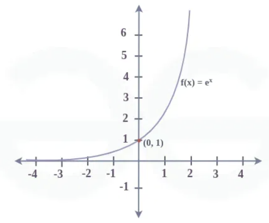
It takes numbers that are negative or that are positive, if you plug in negative numbers you will always get numbers lower than one going down to 0 and if you plug in numbers that are greater than 0 you will get numbers that are greater than 1 going all the way to infinity.
So basically we will take our numbers here:
tensor([[-0.8083, -0.1806,  0.5411, -1.9709, -1.2911,  1.3638, -0.9198, -1.3197,
         -0.9731,  0.9335,  0.2360, -0.4966,  0.0081, -0.5114, -0.6180,  0.6707,
         -0.8448, -0.1883, -0.4675,  1.5044, -1.0876,  0.8690, -0.3955,  1.1926,
          0.0316,  0.2621,  0.3415],
        [ 0.2961,  1.5788, -0.8755,  1.9271, -0.5709, -0.8015,  1.3536,  1.5452,
         -0.5915,  1.0872,  0.6926, -0.2932, -0.3504,  0.7362,  1.2180,  1.3265,
          0.3844, -0.5124,  1.6314,  1.2731,  0.2277, -0.5313, -0.6138, -1.1063,
         -0.8269,  0.2015,  0.6057],
        [-0.0222, -1.4024,  0.4644,  0.2770, -0.7199, -0.8828, -0.3808, -0.2096,
         -0.4294,  0.1786,  1.4026, -0.1493,  0.1361, -0.8037,  1.1314,  0.6296,
          0.0190,  0.3452,  0.0964, -0.6982, -1.0523, -0.6096,  0.0186,  0.7593,
         -0.9675, -0.8365, -1.7953],
        [-0.0222, -1.4024,  0.4644,  0.2770, -0.7199, -0.8828, -0.3808, -0.2096,
         -0.4294,  0.1786,  1.4026, -0.1493,  0.1361, -0.8037,  1.1314,  0.6296,
          0.0190,  0.3452,  0.0964, -0.6982, -1.0523, -0.6096,  0.0186,  0.7593,
         -0.9675, -0.8365, -1.7953],
        [-1.0084, -1.0732,  0.5935,  1.1916,  0.2834,  0.0133, -1.7421,  0.1414,
         -0.2923, -0.0698, -2.5844,  0.8936, -0.2841, -0.9766, -0.6943,  0.8469,
         -0.8529,  0.9908,  0.0906,  0.2939,  0.6630, -0.5760,  0.5404,  1.1129,
         -2.4166, -0.5970,  0.8983]])
and instead of them being positive and negative and all over the place we will interpret them as log counts and then we are going to element-wise exponentiate these numbers like this (xenc @ W).exp() which gives us numbers like these:
tensor([[1.2820, 0.7955, 0.8781, 0.4869, 0.6827, 1.0854, 2.8285, 0.3899, 0.6287,
         1.7204, 0.5149, 0.6895, 1.7907, 0.4574, 1.3713, 0.7026, 1.5253, 4.6257,
         0.5706, 0.5518, 3.1880, 0.2433, 0.7069, 0.0800, 1.6881, 0.4953, 0.7437],
        [0.3695, 1.7570, 0.7501, 0.8455, 3.0995, 0.2958, 1.8581, 0.8969, 0.3401,
         1.4336, 3.0288, 2.2562, 0.6341, 0.4799, 0.5266, 0.4435, 1.2341, 1.4053,
         0.7231, 6.9362, 0.6709, 0.9020, 0.7148, 1.1969, 0.8893, 0.4162, 9.3198],
        [0.0343, 0.8152, 0.6352, 0.3720, 0.1288, 1.6371, 1.3451, 5.2858, 0.8096,
         3.0988, 0.4229, 0.4066, 0.3979, 0.6866, 0.8490, 0.7120, 3.9216, 1.9520,
         0.0717, 0.1542, 1.3433, 2.9977, 0.3933, 2.4173, 0.2609, 0.1910, 0.7122],
        [0.0343, 0.8152, 0.6352, 0.3720, 0.1288, 1.6371, 1.3451, 5.2858, 0.8096,
         3.0988, 0.4229, 0.4066, 0.3979, 0.6866, 0.8490, 0.7120, 3.9216, 1.9520,
         0.0717, 0.1542, 1.3433, 2.9977, 0.3933, 2.4173, 0.2609, 0.1910, 0.7122],
        [0.3095, 0.2317, 0.1807, 0.7596, 0.2873, 0.6711, 3.5370, 0.5818, 4.6902,
         5.0421, 0.1183, 1.6192, 0.5545, 1.1394, 4.4005, 5.9697, 0.2898, 1.6210,
         3.5760, 0.2870, 0.3515, 0.6995, 0.4067, 0.6364, 1.5235, 1.2959, 0.4909]])
You can see that because these numbers went through an exponent, the negative numbers are below 1 and all the originally positive numbers turned into even more positive numbers. These exponentiated outputs here basically give us something that we can use and interpret as the equivalent of counts originally.
We will store these log counts in a variable called logits and then the exponentiated counts in their own variable. Now the probabilities are just the counts normalised.
logits = xenc @ W
counts = logits.exp()
probs = counts / counts.sum(1, keepdim=True)
Each row in probs now sums to 1 and its shape if 5x27, so really what we have achieved is for every 1 our of our 5 examples we now have a row that came out of a neural net and because of our transformations we made sure that the output of our neural net are probabilities or at least we can interpret to be probabilities. So again, our wx gave us logits and then we interpret those to be log counts, we exponentiate to get something that looks like counts and then we normalise those counts to get a probability distribution. All of these are differentiable operations.
For example, for the 0th example probs[0] we see this:
tensor([0.0312, 0.0074, 0.0623, 0.0179, 0.0132, 0.0108, 0.0108, 0.0060, 0.0252,
        0.0350, 0.0321, 0.0053, 0.0393, 0.0120, 0.0044, 0.2400, 0.0583, 0.0033,
        0.1966, 0.0193, 0.0090, 0.0121, 0.0203, 0.0014, 0.0671, 0.0077, 0.0522])
Which is where we fed in 0 which corresponds to the dot, and again the way we did that is we first got its index, then we one hot encoded it, then it went into the neural net and out came this distribution of probabilities, and its shape is 27 long, we will interpret this as the neural net's assignment for how likely every one of these 27 characters are to come next. And as we tune the weights W we will be getting different probabilities out for any character that you input. So now the question is just can you optimise and find a good W such that the probabilities coming out are pretty good, and the way we measure pretty good is by the loss function.
Ok let's organise everything and summarise a little, so it starts here with our input dataset xs:
tensor([ 0, 5, 13, 13, 1])and we also have some labels ys for the correct next character in a sequence, and these are integers:
tensor([ 5, 13, 13, 1, 0])Here:
g = torch.Generator().manual_seed(2147483647)
W = torch.randn((27, 27), generator=g)
I am using torch generators so that you see the same numbers that I see. I'm generating 27 neurons' weights and each neuron receives 27 inputs.
xenc = F.one_hot(xs, num_classes=27).float() # input to the network: one-hot encoding
logits = xenc @ W # predict log-counts
counts = logits.exp() # counts, equivalent to N
probs = counts / counts.sum(1, keepdims=True) # probabilities for next character
Now here we are going to plug in all the input examples xs into a neural net, this is the forward pass. First we encode all of the inputs into one hot representations, so xenc becomes an array that is 5x27 (mosly 0s except for a few 1s). We then multiply this in the first layer of a neural net to get logits, exponentiate the logits to get fake counts and then normalise these counts to get probabilities.
Those last two lines are actually called a softmax
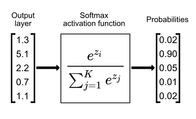
Softmax is a very often used layer in a neural net that takes these z values which are logits, exponentiates them and divides and normalises. It's a way of taking outputs of a neural net layer, where the outputs can be positive of negative and it outputs probability distributions, its outputs always sum to 1 and are all positive, just like probabilities.
Now you should notice that this entire forward pass is made up of differentiable layers everything here we can backpropogate through.
Now we achieve these probabilities which are 5x27 for every single example we have a vector of probabilities that sums to 1 and then here I wrote a bunch of stuff to kind of like break down the example:
nlls = torch.zeros(5)
for i in range(5):
  # i-th bigram:
  x = xs[i].item() # input character index
  y = ys[i].item() # label character index
  print('--------')
  print(f'bigram example {i+1}: {itos[x]}{itos[y]} (indexes {x},{y})')
  print('input to the neural net:', x)
  print('output probabilities from the neural net:', probs[i])
  print('label (actual next character):', y)
  p = probs[i, y]
  print('probability assigned by the net to the the correct character:', p.item())
  logp = torch.log(p)
  print('log likelihood:', logp.item())
  nll = -logp
  print('negative log likelihood:', nll.item())
  nlls[i] = nll

print('=========')
print('average negative log likelihood, i.e. loss =', nlls.mean().item())
and its output looks like this:
--------
bigram example 1: .e (indexes 0,5)
input to the neural net: 0
output probabilities from the neural net: tensor([0.0607, 0.0100, 0.0123, 0.0042, 0.0168, 0.0123, 0.0027, 0.0232, 0.0137,
        0.0313, 0.0079, 0.0278, 0.0091, 0.0082, 0.0500, 0.2378, 0.0603, 0.0025,
        0.0249, 0.0055, 0.0339, 0.0109, 0.0029, 0.0198, 0.0118, 0.1537, 0.1459])
label (actual next character): 5
probability assigned by the net to the the correct character: 0.012286250479519367
log likelihood: -4.3992743492126465
negative log likelihood: 4.3992743492126465
--------
bigram example 2: em (indexes 5,13)
input to the neural net: 5
output probabilities from the neural net: tensor([0.0290, 0.0796, 0.0248, 0.0521, 0.1989, 0.0289, 0.0094, 0.0335, 0.0097,
        0.0301, 0.0702, 0.0228, 0.0115, 0.0181, 0.0108, 0.0315, 0.0291, 0.0045,
        0.0916, 0.0215, 0.0486, 0.0300, 0.0501, 0.0027, 0.0118, 0.0022, 0.0472])
label (actual next character): 13
probability assigned by the net to the the correct character: 0.018050704151391983
log likelihood: -4.014570713043213
negative log likelihood: 4.014570713043213
--------
bigram example 3: mm (indexes 13,13)
input to the neural net: 13
output probabilities from the neural net: tensor([0.0312, 0.0737, 0.0484, 0.0333, 0.0674, 0.0200, 0.0263, 0.0249, 0.1226,
        0.0164, 0.0075, 0.0789, 0.0131, 0.0267, 0.0147, 0.0112, 0.0585, 0.0121,
        0.0650, 0.0058, 0.0208, 0.0078, 0.0133, 0.0203, 0.1204, 0.0469, 0.0126])
label (actual next character): 13
probability assigned by the net to the the correct character: 0.026691533625125885
log likelihood: -3.623408794403076
negative log likelihood: 3.623408794403076
--------
bigram example 4: ma (indexes 13,1)
input to the neural net: 13
output probabilities from the neural net: tensor([0.0312, 0.0737, 0.0484, 0.0333, 0.0674, 0.0200, 0.0263, 0.0249, 0.1226,
        0.0164, 0.0075, 0.0789, 0.0131, 0.0267, 0.0147, 0.0112, 0.0585, 0.0121,
        0.0650, 0.0058, 0.0208, 0.0078, 0.0133, 0.0203, 0.1204, 0.0469, 0.0126])
label (actual next character): 1
probability assigned by the net to the the correct character: 0.07367684692144394
log likelihood: -2.6080667972564697
negative log likelihood: 2.6080667972564697
--------
bigram example 5: a. (indexes 1,0)
input to the neural net: 1
output probabilities from the neural net: tensor([0.0150, 0.0086, 0.0396, 0.0100, 0.0606, 0.0308, 0.1084, 0.0131, 0.0125,
        0.0048, 0.1024, 0.0086, 0.0988, 0.0112, 0.0232, 0.0207, 0.0408, 0.0078,
        0.0899, 0.0531, 0.0463, 0.0309, 0.0051, 0.0329, 0.0654, 0.0503, 0.0091])
label (actual next character): 0
probability assigned by the net to the the correct character: 0.01497753243893385
log likelihood: -4.2012038230896
negative log likelihood: 4.2012038230896
=========
average negative log likelihood, i.e. loss = 3.7693049907684326
So we have 5 examples making up 'emma' and there are 5 bigrams inside 'emma'. So bigram example 1 is that e is the beginning character .e right after dot. The indexes for these are 0 and 5, so we feed in a zero and we get probabilities from the neural net that are 27 numbers:
tensor([0.0290, 0.0796, 0.0248, 0.0521, 0.1989, 0.0289, 0.0094, 0.0335, 0.0097,
        0.0301, 0.0702, 0.0228, 0.0115, 0.0181, 0.0108, 0.0315, 0.0291, 0.0045,
        0.0916, 0.0215, 0.0486, 0.0300, 0.0501, 0.0027, 0.0118, 0.0022, 0.0472])
And then the label is 5, because it is e that comes after the dot, so that's the label, and then we use this label 5 to index into the probability distribution here and we see this probability in its place: 0.012286250479519367, so this is the probabiilty assigned by the neural net to the actual correct character, it tells me that the network thinks that the e is only 1% likely to follow, which is of course not very good because this is a training example and the network thinks this is very very unlikely. But that's just because we didn't get very lucky in generating a good setting of W.
So the log likelihood is very negative: -4.3992743492126465 and then negative log likelihood is very positive: 4.3992743492126465, this is very high and this means that we are going to have a high loss which is just the average negative log likelihood. And this repeats and is done for the other bigrams.
Overall we can see that the average negative log likelihood which is the loss is 3.7693049907684326, so the total loss that basically summarises how well this network currently works (at least on this one word) is a very high loss.
Now we could go and change the generator to randomly guess and use different values and see if that lowers our loss but that is a terrible way to go about lowering the loss. The way we actually optimise a neural net is we start with some random guess and we use the loss which is again made up of only differentiable operations and we can minimise the loss by tuning W, by computing the gradients of the loss with respect to these W matrices. So we just tune W to minimise the loss and find a good setting of W using gradient based optimisation, so let's see how that will work.
Now, if you have read or seen my implementation of zdravkograd then you might notice that things from now are going to look very similar. So we have done our forward pass and now we have to evaluate our loss, we are not using the mean squared error like we did in zdravkograd but rather the negative log likelihood because we are doing classification, we are not doing regression (which we did in zdravkograd).
probs.shape is torch.Size([5, 27]) and so we basically want to pluck out the probabilities at the correct indices here and we use the labels ys for this. So for the first example we are looking at the probability of 5 so we use probs[0, 5], for the second row we are interested in this one probs[1, 13] and so on. We need these probabilities:
probs[0, 5], probs[1, 13], probs[2, 13], probs[3, 1], probs[4, 0]So these are the probabilities we are interested in:
(tensor(0.0123),
 tensor(0.0181),
 tensor(0.0267),
 tensor(0.0737),
 tensor(0.0150))
and you can see that they are not amazing, but still we want a more efficient way to access these probabilities, not just listing them out like this. The way to do this in PyTorch, or one of the ways at least, is that we can basically pass in all of these integers in vector form. These first ones, 0 through 4, we can actually just create that using torch.arange(5) which outputs tensor([0, 1, 2, 3, 4]). So we can index here with probs[torch.arange(5), ys] and the second part is just the ys. That gives us tensor([0.0123, 0.0181, 0.0267, 0.0737, 0.0150]), which is the same as we had previously. This plucks out the probabilities that the neural network assigns to the correct next character.
Now we take those probabilities and we actually look at the log of them, so we .log() and then we want to average that out, so take the .mean() of all that, and it's the negative of all that also that is the loss.
loss = -probs[torch.arange(5), ys].log().meanwhich turns out to be very bad: tensor(3.7693). Ok that's fine, we have now done the forward pass and we also have the loss, now we are ready to do the backward pass.
We want to first make sure that all the gradients are reset so they're at 0. Now in PyTorch you can set them to 0 but you can also set them to None and setting it to None is more efficient. Now we do loss.backward(), but before we do this we need one more thing, if you remember from zdravkograd PyTorch actually requires that we set requires_grad=True here W = torch.randn((27, 27), generator=g, requires_grad=True) so that we tell PyTorch that we are interested in calculating the gradients for this leaf tensor and by default this is false.
# backward pass
W.grad = None
loss.backward()
Something magical happened when we ran this, PyTorch, just like zdravkograd, when we did the forward pass earlier it keeps track of all the operations under the hood, it builds a full computational graph, just like the graphs we produced in zdravkograd those graphs exist inside PyTorch and so it knows all the dependencies and all the mathematical operations of everything and when you then calculate the loss we can call this .backward() on it. This then fills in the gradients of all the intermediates all the way back to W. Now, our W.grad has structure, theres stuff inside it. Now every element of W.grad is telling us the influence of that weight on the loss function. So we can use this gradient information to update the weights of this neural network, so let's now do that update.
W.data += -0.1 * W.gradSo we update the tensor like that. So if we print the loss right now we see 3.7693049907684326, we have also now updated W so if I recalc the forward pass the loss should be slightly lower. So 3.7693049907684326 goes to 3.7492129802703857, and repeating that is gradient descent. When we achieve a low loss that means the network is assigning high probabilities to the correct next character.
Ok now let's rearrange everything and put it all together one last time:
# create the dataset
xs, ys = [], []
for w in words[:1]:
  chs = ['.'] + list(w) + ['.']
  for ch1, ch2 in zip(chs, chs[1:]):
    ix1 = stoi[ch1]
    ix2 = stoi[ch2]
    xs.append(ix1)
    ys.append(ix2)
xs = torch.tensor(xs)
ys = torch.tensor(ys)
num = xs.nelement()
print('number of examples: ', num)

# initialize the 'network'
g = torch.Generator().manual_seed(2147483647)
W = torch.randn((27, 27), generator=g, requires_grad=True)
So here is where we construct our dataset of bigrams, you see that we are still only iterating over the first word, emma, we will change that in a second. I added a num that counts the number of elements in xs, so that we can see explicitly that number of examples if 5, because we are currently just working with emma.
# gradient descent
for k in range(10):

    # forward pass
    xenc = F.one_hot(xs, num_classes=27).float() # input to the network: one-hot encoding
    logits = xenc @ W # predict log-counts
    counts = logits.exp() # counts, equivalent to N
    probs = counts / counts.sum(1, keepdims=True) # probabilities for next character
    loss = -probs[torch.arange(num), ys].log().mean()
    print(loss.item())

    # backward pass
    W.grad = None
    loss.backward()

    # update
    W.data += -0.1 * W.grad
And then here I added a loop of exactly what we had before, so we had 10 iterations of gradient descent (forward pass, backward pass and then update). And so running these two cells, initialisation and gradient descent gives us:
3.7693049907684326
3.7492129802703857
3.7291626930236816
3.7091546058654785
3.6891887187957764
3.66926646232605
3.6493873596191406
3.6295523643493652
3.6097614765167236
3.5900158882141113
It gives us some improvement on the loss function. But now I want to use all the words, and there's not 5 but rather 228146 bigrams now, and all the code we wrote doesn't care if theres 5 bigrams or 228146 bigrams, so it should work without any issues.
3.758953094482422
3.758040189743042
3.757127523422241
3.756216049194336
3.755305767059326
3.754396915435791
3.753488779067993
3.7525813579559326
3.7516753673553467
3.750770330429077
And so we get these results, we are decreasing very slightly so actually we can probably afford a larger learning rate like 1:
3.749866485595703
3.6621599197387695
3.5838623046875
3.513427972793579
3.44982647895813
3.392310619354248
3.340266227722168
3.293151378631592
3.2504563331604004
3.211688995361328
Ok we can probably afford an even larger learning rate of 10:
3.176388740539551
3.144124746322632
3.1145212650299072
3.0872490406036377
3.0620319843292236
3.0386369228363037
3.0168704986572266
2.996567964553833
2.977591037750244
2.9598190784454346
What if we bump it up to 50:
3.758953094482422
3.371079444885254
3.1540327072143555
3.0203664302825928
2.9277069568634033
2.8604001998901367
2.809727191925049
2.7701010704040527
2.738072633743286
2.711496114730835
It's still working! Even 50 seems to work. So let's re-initialise and let's run 100 iterations:
3.758953094482422
3.371079444885254
3.1540327072143555
3.0203664302825928
2.9277069568634033
2.8604001998901367
2.809727191925049
2.7701010704040527
2.738072633743286
2.711496114730835
2.6890029907226562
2.6696884632110596
2.6529300212860107
2.638277053833008
2.6253879070281982
2.613990306854248
2.60386323928833
2.5948216915130615
2.586712121963501
2.579403877258301
2.572789192199707
2.5667762756347656
2.5612881183624268
2.5562589168548584
2.551633596420288
...
2.4735772609710693
2.4733383655548096
2.47310471534729
2.4728763103485107
Some pretty good losses, let me run 100 more (also what is the number we are expecting?):
2.4726529121398926
2.4724342823028564
2.4722204208374023
2.472011089324951
2.4718058109283447
2.4716055393218994
2.471409320831299
2.4712166786193848
2.4710280895233154
2.47084379196167
2.4706625938415527
2.4704854488372803
2.470311403274536
2.4701414108276367
2.4699742794036865
2.4698104858398438
2.4696500301361084
2.4694924354553223
2.4693379402160645
2.4691860675811768
2.4690370559692383
2.468891143798828
2.468747615814209
2.46860671043396
2.468468427658081
...
2.462538242340088
2.462489128112793
2.4624407291412354
2.462392807006836
Well we are expecting to get something around what we had originally actually. So all the way back, if you remember in the beginning when we optimised just by counting our loss was roughly 2.47... after we added smoothing, and so that's actually roughly the vicinity of what we expect to achieve, but before we achieved it by counting and here we are trying to achieve it with gradient based optimisation rather than counting. So we come to about 2.46.
That makes sense because fundamentally we are not taking in any additional information, we are still just taking in the previous character and trying to predict the next one but instead of doing it explicitly by counting and normalising we are doing it with gradient based learning. It just so happens that the explicit approach happens to very well optimise the loss function without any need for gradient based optimisation because the setup for bigram language models is so simple that we can just afford to estimate those probabilities directly and maintian them in a table.
However, the gradient based approach is significantly more flexible, so we've actually gained a lot because now we can expand this approach and complexify the neural network. Currently we are just taking a single character and feeding into a neural net and this neural net is extremely simple but we are about to iterate on this substantially. We will be taking multiple previous characters and we are going to be feeding them into increasingly more complex neural nets but fundamentally the output of the neural net will always just be logits and those logits will go through the exact same transformation. We will take them through a softmax, calculate the loss function and the negative log likelihood and then do gradient based optimisation.
So actually, as we complexify the neural nets and work all the way up to transformers none of this code will really fundamentally change, the only thing that will change is the way we do the forward pass where we take in some previous characters and calculate logits for the next character in a sequence. That part will become more complex but we will use the same machinery to optimise it. It's not obvious how we would have extended the initial bigram approach in the case where there are many more characters at the input because eventually the tables would get way too large because there's way too many combinations of what the previous characters could be. If you only have one previous character we can just keep everything in a table, but if you have the last 10 characters of an input we can't actually keep everything in a table anymore, so it is fundamentally an unscalable approach. The NN approach is significantly more scalable and it's something that we can improve on over time.
I also want to point out 2 more things.
Number 1, if you take a look at this line of code from above:
logits = xenc @ W # predict log-countsNotice that this xenc here is made up of one hot vectors and this is multiplied this W matrix, we think of this as multiple neurons being forwarded in a fully connected manner. But actually what's happening here is if you have a one hot vector here that has a 1 in say the 5th dimension then because of the way the matrix multiplication works, multiplying that one hot vector with W, actually ends up plucking out the 5th row of W. Logits would become just the 5th row of W. The interesting thing is that that is exactly what was happening before, remember all the way before we had a bigram, we took the first character and that first character indexed into a row of our massive table and that row gave us the probability distribution for the next character. So te first character was used as a lookup into a matrix to get the probability distribution. That is exactly what is happening now too, because we are taking the index, encoding it as one hot and multiplying it by W, so logits literally becomes the appropriate row of W and that gets, just as before, exponentiated to get the counts and then normalised and becomes probabilities.
So W is literally the same as the massive table array we had earlier, but W is the log counts not the counts, so it's more precise to say that W exponentiated is that table. But that previous table was filled in by counting and by populating the counts of bigrams but in the gradient based framework we initialise it randomly and we let the loss guide us to arrive at the exact same array, so the previous table is basically the array W at the end of optimisation except we arrived at it piece by piece by following the loss, and that's why we also obtain the same loss function at the end.
The second note is, remember the smoothing where we added fake counts to our counts in order to smooth out and make more uniform distributions of our probabilities and that prevented us from assigning 0 probability to any one bigram. Now if I increased that count, so it wasn't the 1 we had but something more like 10,000 then the probability becomes more and more uniform. It turns out that the gradient based framework has an equivalent to smoothing. In particular, think about the W's, which we initialised randomly but we could have also initialised all of W's entries to be 0. If they were all 0, then the logits would become all 0 and then exponentiating those logits would turn them all into 1 and then the probabilities turn out to be exactly uniform. So basically, when W is all equal to each other, especially 0, then the probabilities come out to be completely uniform. So trying to incentivise W to be near 0 is basically equivalent to label smoothing and the more you incentivise that in the loss function the more smooth distribution you are going to aschieve.
This brings us to something called Regularisation, where we can actually augment the loss function to have a small component that we call a regularisation loss. In particular what we are going to do, is we are going to take W and we can square all of its entries and then sum them. (W**2).sum(). Because we are squaring there will be no more signs anymore, the way this works is you achieve zero loss if W is exactly or 0 but if W has non zero numbers you accumulate loss. So we can take that and we can add it onto this line:
loss = -probs[torch.arange(num), ys].log().mean() + 0.01*(W**2).mean()And actually instead of sum we will take a mean because otherwise the sum gets too large and it will affect the loss way too much, and we also multiply it by 0.01 and we have a regularisation loss here, you can choose whatever strength you would like. Now if we run this optimisation it has 2 components, not only is it trying to make all the probabilities work out but in addition to that there is an additional component that simultaneously tries to make W's zero, because if W's are non zero you feel a loss and so minimising this is to try to get W to tend towards zero. You can think of this as adding like a spring or gravity force that pushes W to be zero.
Okay and lastly, before I finish up this part, I want to sample from this neural net model:
# finally, sample from the 'neural net' model
g = torch.Generator().manual_seed(2147483647)

for i in range(5):

    out = []
    ix = 0
    while True:
        xenc = F.one_hot(torch.tensor([ix]), num_classes=27).float()
        logits = xenc @ W
        counts = logits.exp()
        P = counts / counts.sum(1, keepdims=True)

        ix = torch.multinomial(P, num_samples=1, replacement=True, generator=g).item()
        out.append(itos[ix])
        if ix == 0:
            break
    print(''.join(out))
This is similar to the code from before that we have already used, remember we sampled 5 times. First we take ix and we encode it into a one hot row of xenc which then multiplies our W (which really just plucks out the row of W corresponding to ix). Now we have our logits and then we normalise those logits, exponentiate to get counts and then normalise to get the distribution and then we can sample from the distribution. So if I run this:
cexze.
momasurailezitynn.
konimittain.
llayn.
ka.
Kind of anticlimactic but we get the exact same result as we did when we sampled from the counting bigram model, that's because this is the exact same model.
Okay and that's it for part 1, I've covered a lot of ground, I learnt the bigram language model, I trained the model, I sampled from the model and I evaluated the quality of the model using the negative log likelihood of the loss. I also trained the model in two completely different ways that actually gave the same result. In the first way, I just counted up the frequency of all the bigrams and normalised and in the second way I used the negative log likelihood loss as a guide to optimising the counts matrix so that the loss is minimised in a gradient based framework. I realised that the second one of these, the gradient based framework is much more flexible, right now my neural network is super simple, it's taking a single previous character and taking it through a single linear layer to calculate the logits, this is about to complexify in part 2. I want to take more and more of these characters and feed them all into a neural net, however this NN will still output the exact same thing: logits. They will still be normalised in the exact same way, everything will stay identical its just that this NN will now complexify all the way to transformers.
Thank you for reading :)