
TLDR:
This is a deep-dive blog post on my journey building a handwritten digit recogniser web app using a neural network I built from scratch. I start with detailed notes on neural network basics (structure, weights, learning via gradient descent/backprop), then cover implementing the model in Python (training on MNIST, exporting to JSON). Finally, I detail the Next.js frontend (grid drawing, mobile fixes, preprocessing for accuracy). Source code on Github, app live on Vercel.
Table of Contents
- Introduction and Motivation
- The Problem
- Learning the Theory – Neural Network Basics
- How the Network Learns
- What is Backpropagation?
- Implementing the Model in Python
- Building the Next.js Web App
- Challenges and Learnings
- The End
Introduction and Motivation
Ok, so I want to build a web app where a user draws a number 0-9 and the computer does bish bash bosh and predicts what number you have drawn. How do you do this? I don't know, so first I gathered knowledge. As mostly a visual learner, I found 3Blue1Brown's videos on the topic very useful on getting an intuitive understanding of the concepts, I made some notes on these videos so I wasn't just passively learning. To then get deeper into it, I read Michael Nielsen's Neural Networks and Deep Learning book, it really helped having the intuitive knowledge from the videos beforehand.
My motivation? Pure curiosity about how machine learning really works, plus a cool portfolio project. Knowledge gained is the ammo, motivation is my gun, now let's shoot it straight into the problem at hand.
The Problem
How is it that our brain can see a number 3 and know it's a number 3? That's crazy because you can look at one 3 written one way and another 3 written a completely different way, could even be doctor's handwriting and still your brain would know what number it is!
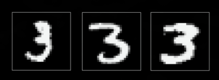
Essentially, my task is to write some code that would mimic what the brain is doing, it would be taking in an image of a number (drawn by a user) and resolving it to a digit from zero to nine. This super trivial task that our brain does now becomes quite tricky when you have to turn it into code.
Learning the Theory – Neural Network Basics
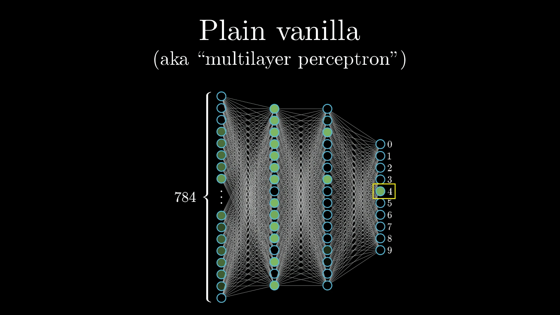
Alright, so we will use a neural network to solve this problem, but first of all, what is a neural network? Well, there are many variants, for example convolutional neural networks (CNN), recurrent neural networks (RNN), transformers, and many more. But let's start by learning about the most basic one of them all, the plain vanilla form of a neural network.
Neurons
To break it down super simply, a neuron is a thing that holds a number, that's it, specifically a number between 0 and 1.
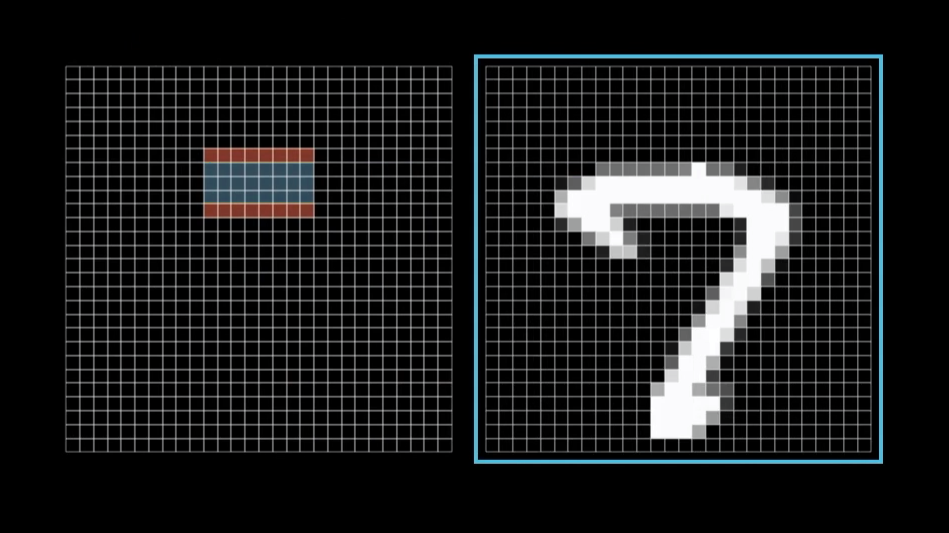
For example, our images will be 28x28 pixels meaning we will have 784 neurons, each of which holds a number. This number corresponds to its greyscale value of the pixel, 0 for black and up to 1 for white ones.

You could think of this as being analogous to how neurons in the brain can be active or inactive.
All of our images will be 28x28 pixels, in total 784 pixels, each with a brightness value between 0.0 and 1.0. To represent this in the network, we create a layer of 784 neurons where each neuron corresponds to a particular pixel.
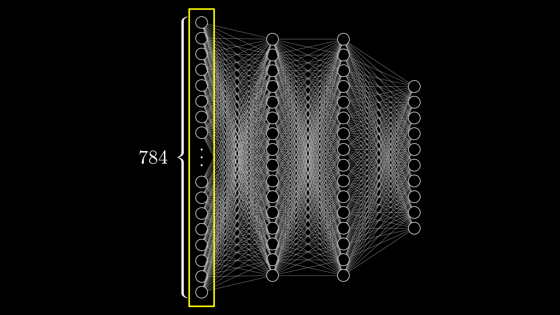
That's our first layer, called the input layer, done. Now when we want to pass an image into the network, we'll set each input neuron's activation to the brightness of the corresponding pixel.
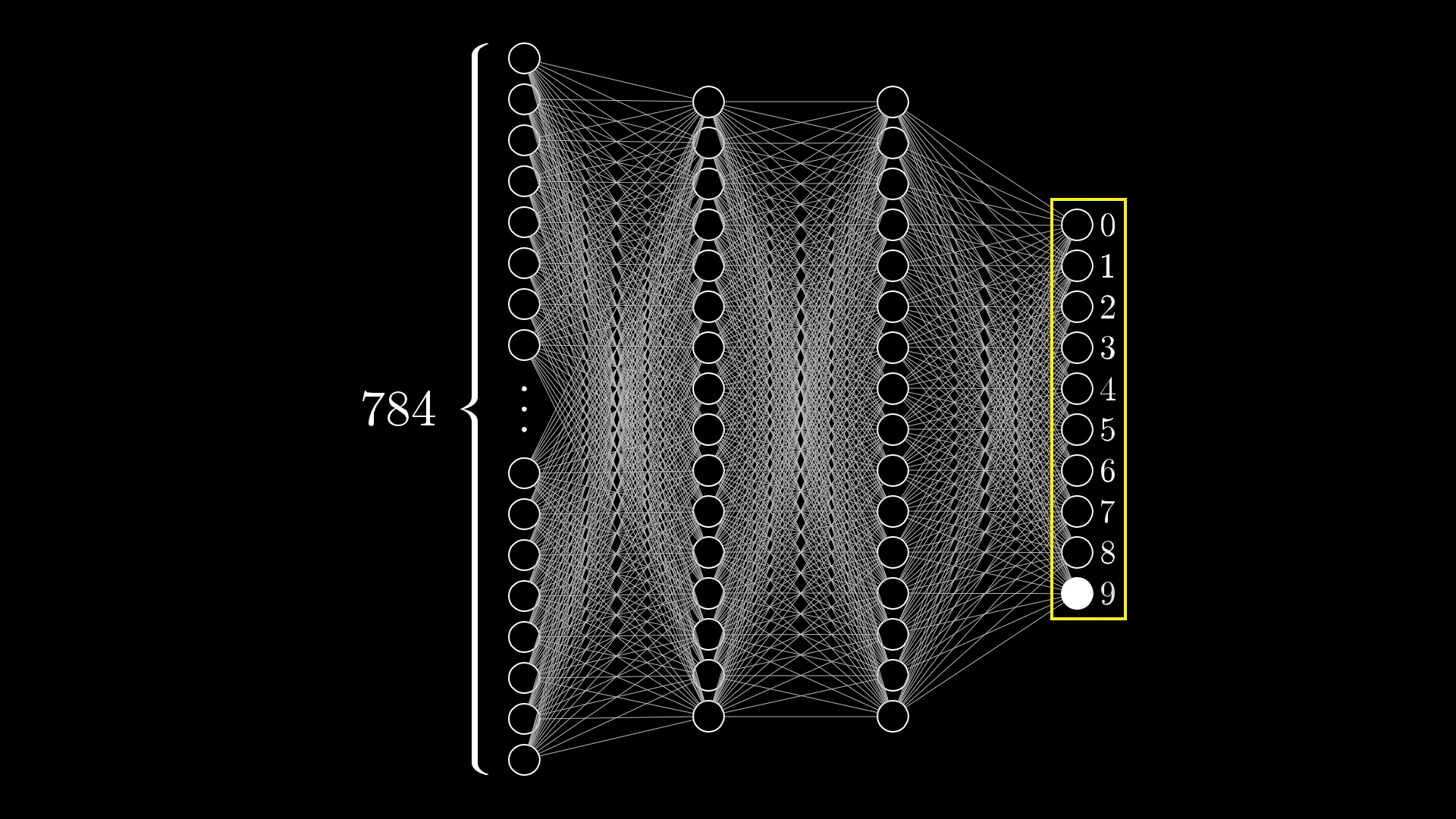
Now let's jump over to the last layer of our network, it will have 10 neurons, each one representing one of the possible digits. The activation in these neurons, again between 0.0 and 1.0, will represent how much the system thinks an image corresponds to a given digit.
The Hidden Layers
There are also a couple of layers in between called the "hidden layers", don't worry about these for now but do know that they exist.
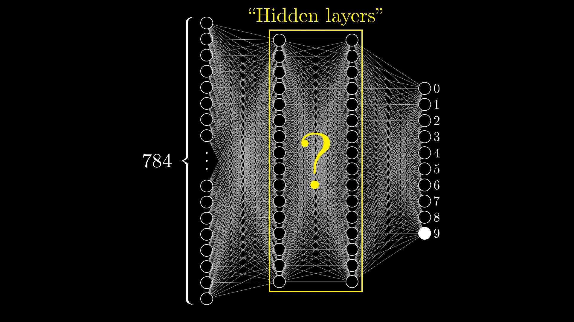
Here you can see two hidden layers each with 16 neurons. Why these choices? Completely arbitrary, but also 16 is just a nice number.
You will notice how in these drawings each neuron from one layer is connected to each neuron from the next. This is because activations in one layer determine the activations in the next layer.
However, not all of these connections are equal, some are stronger than others and determining how strong these connections are is the heart of how neural networks operate.
Before we jump into the maths behind them let's think a little bit more broadly about how we might expect a layered structure like this to behave.
When you or I recognise digits we piece together various different components like loops and lines, so each digit can be broken down into smaller recognisable structures.
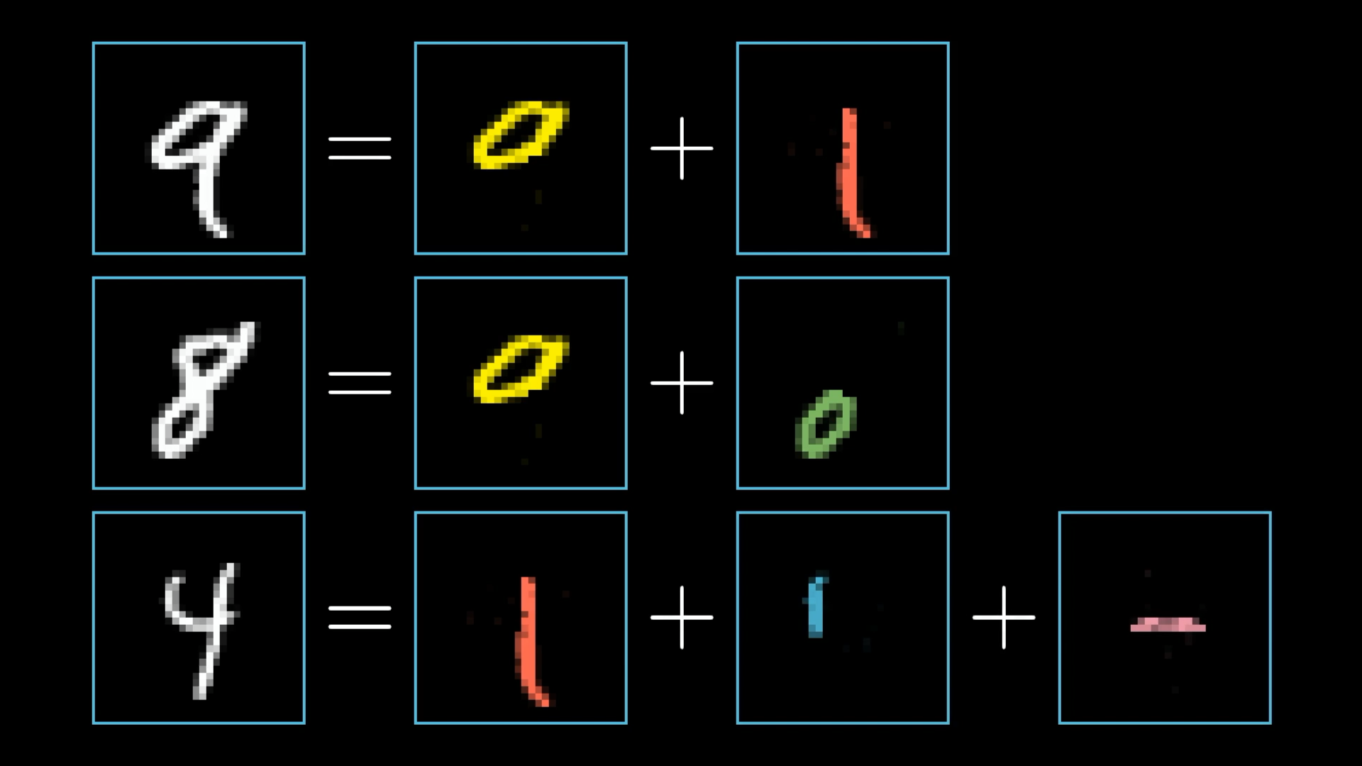
In an ideal scenario we might hope that each neuron in the second to last layer corresponds to one of these subcomponents. Such that anytime you feed an image with a loop up top, there is some specific neuron whose activation will be close to 1.0.
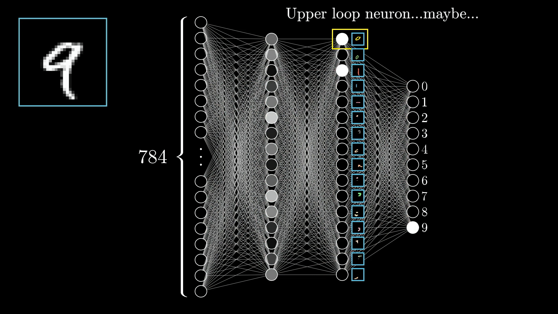
And not just that exact loop of pixels. The hope would be that any generally loopy pattern towards the top of image sets off this neuron. That way, going from the third layer to the last one would just require learning which combinations of subcomponents correspond to which digits.
But how do you even recognise these subcomponents? Well recognising a loop can also be broken down into subproblems. One reasonable way to do that would be to first recognise the various edges that make it up.
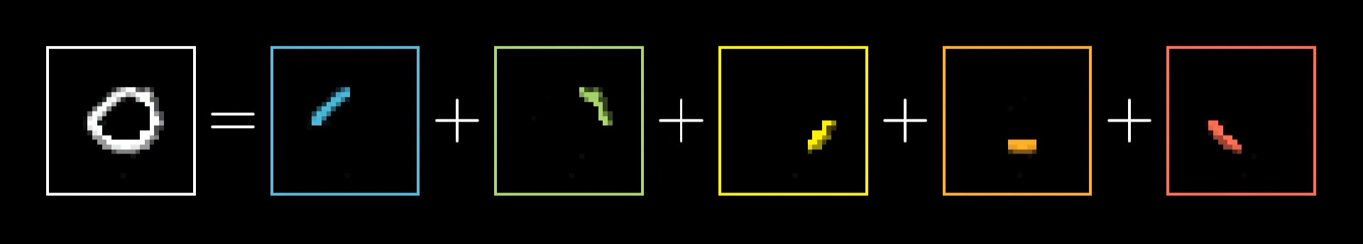
In the same way, long lines, like those found in the digits 1, 4, or 7, can be thought of as a single extended edge, or perhaps as a specific arrangement of multiple shorter edges.
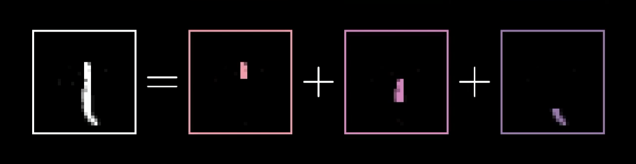
You can think of it like this, maybe each neuron in the second layer is tuned to spot a tiny edge somewhere in the image, so when you show the network a picture, those neurons light up for all the little edges they find, then the third layer picks up on bigger patterns, like loops or long lines, and finally, one of the neurons in the last layer gets excited if it thinks the image matches a certain digit.
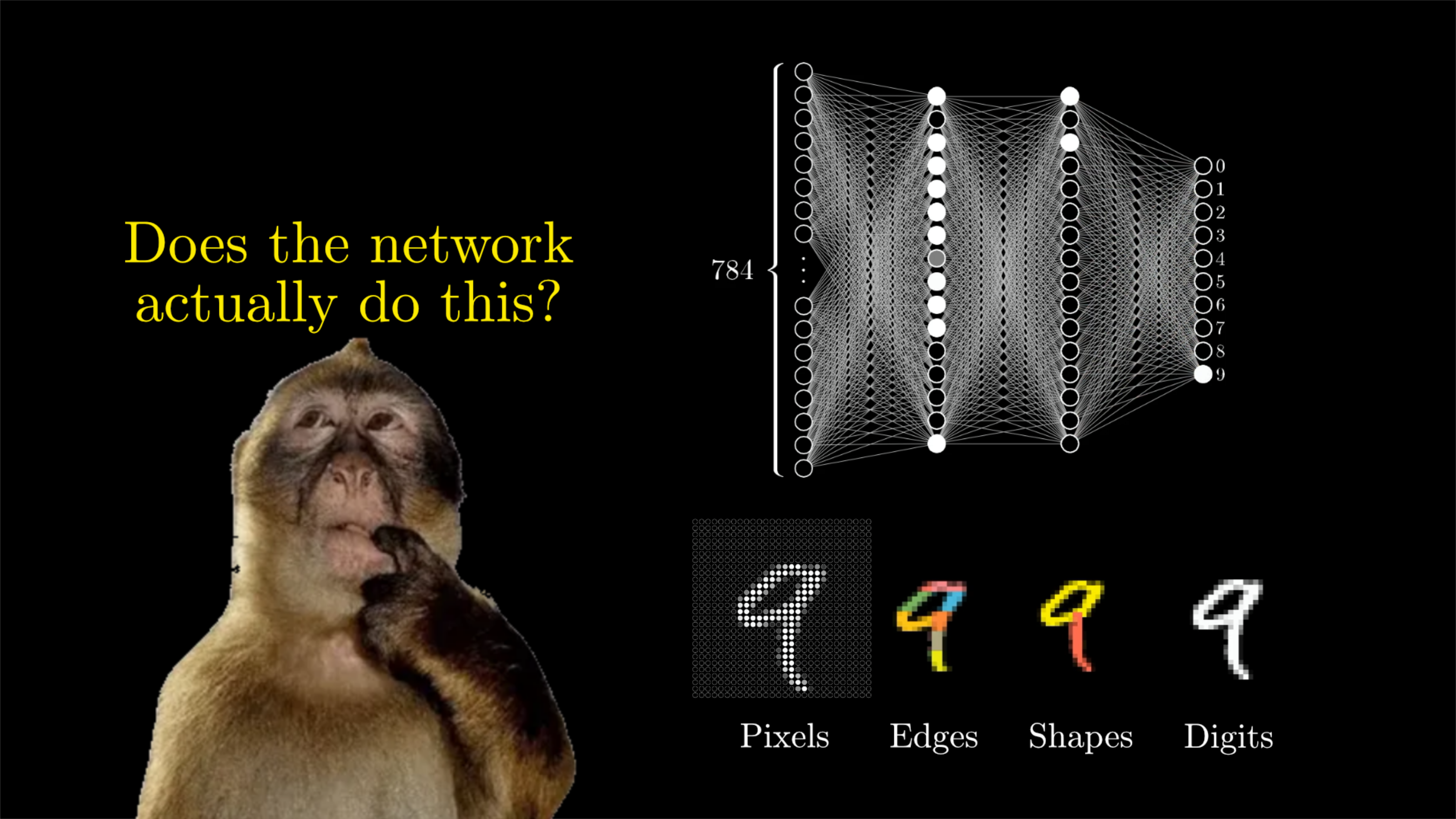
Of course, there's no guarantee that our network will end up working exactly this way, but it's a reasonable expectation to have in mind as we design it.
Layers Break Problems into Bite Sized Pieces
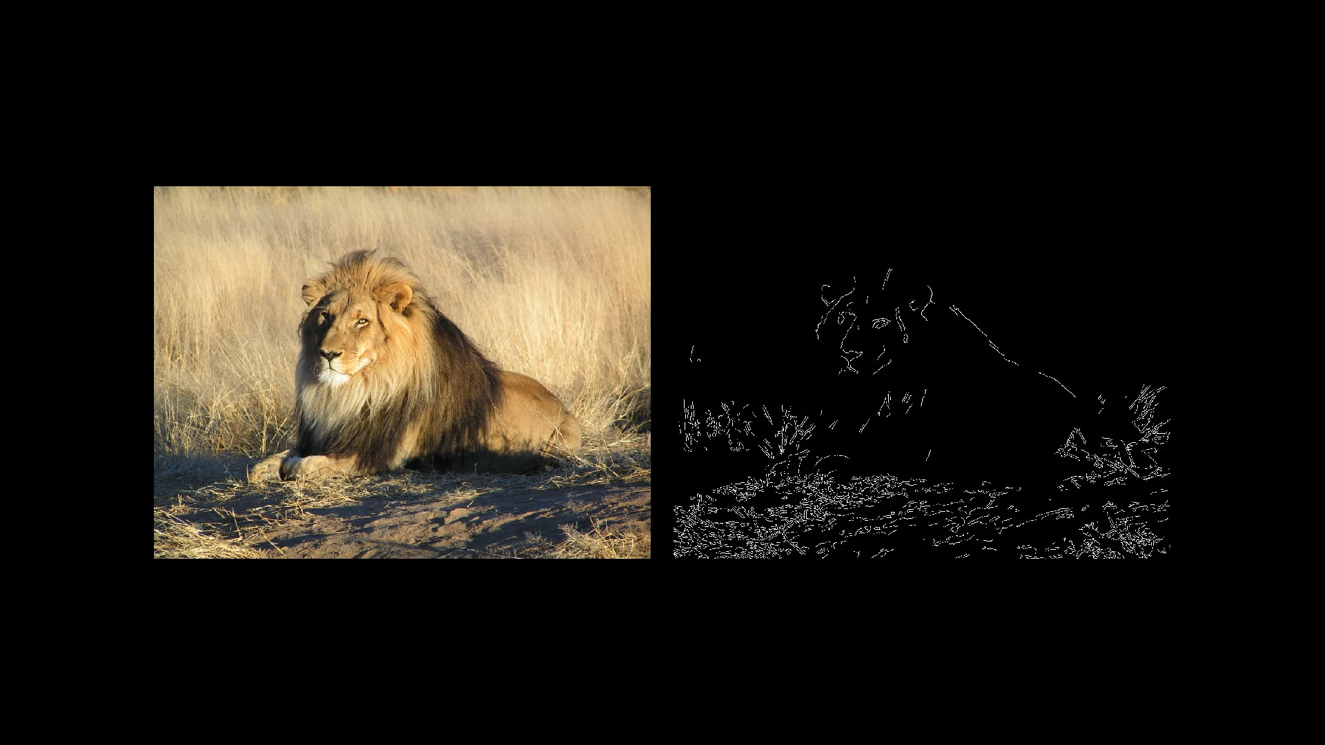
You can imagine how being able to detect edges and patterns would also be useful for other image recognition tasks.
And it’s not just about image recognition, you can actually break down all kinds of smart tasks into layers like this. Take speech, for instance, you start with raw audio, then pick out individual sounds, those sounds come together to make syllables, which then form words, and those words build up into phrases and even more complex ideas.
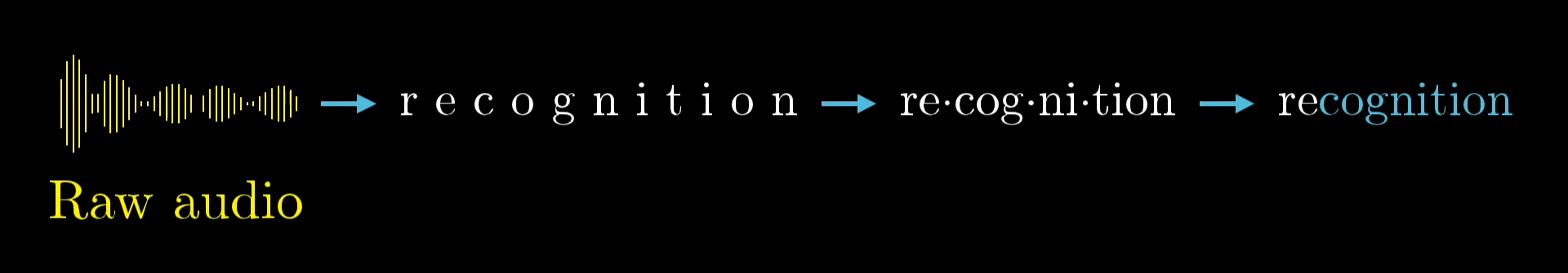
What’s really nice about having layers in a neural network is that it helps you tackle tough problems by breaking them into smaller, more manageable pieces, making it much easier to move from one layer to the next.
How Information Passes Between Layers
Alright, so now that we have this general idea in mind, how would you actually go about building it? What we really want is some way to take the raw pixels and combine them into edges, then combine those edges into bigger patterns, and finally turn those patterns into digits. It would be really neat if each of these steps could use the same kind of maths, making the whole process feel unified and simple.
let's zoom in on one very specific example, say that the hope is for this one particular neuron in the second layer to pick up on whether or not the image has an edge in this spot here:
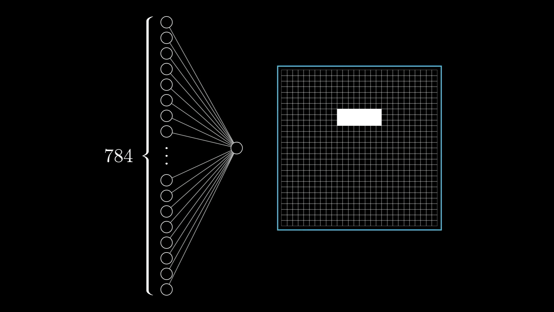
With this in mind, what parameters do you think the network should have, what knobs and dials should you be able to tweak so that it's expressive enough to potentially capture this pattern? Or other pixel patterns, like for example the pattern that several edges can make a loop, and other such things.
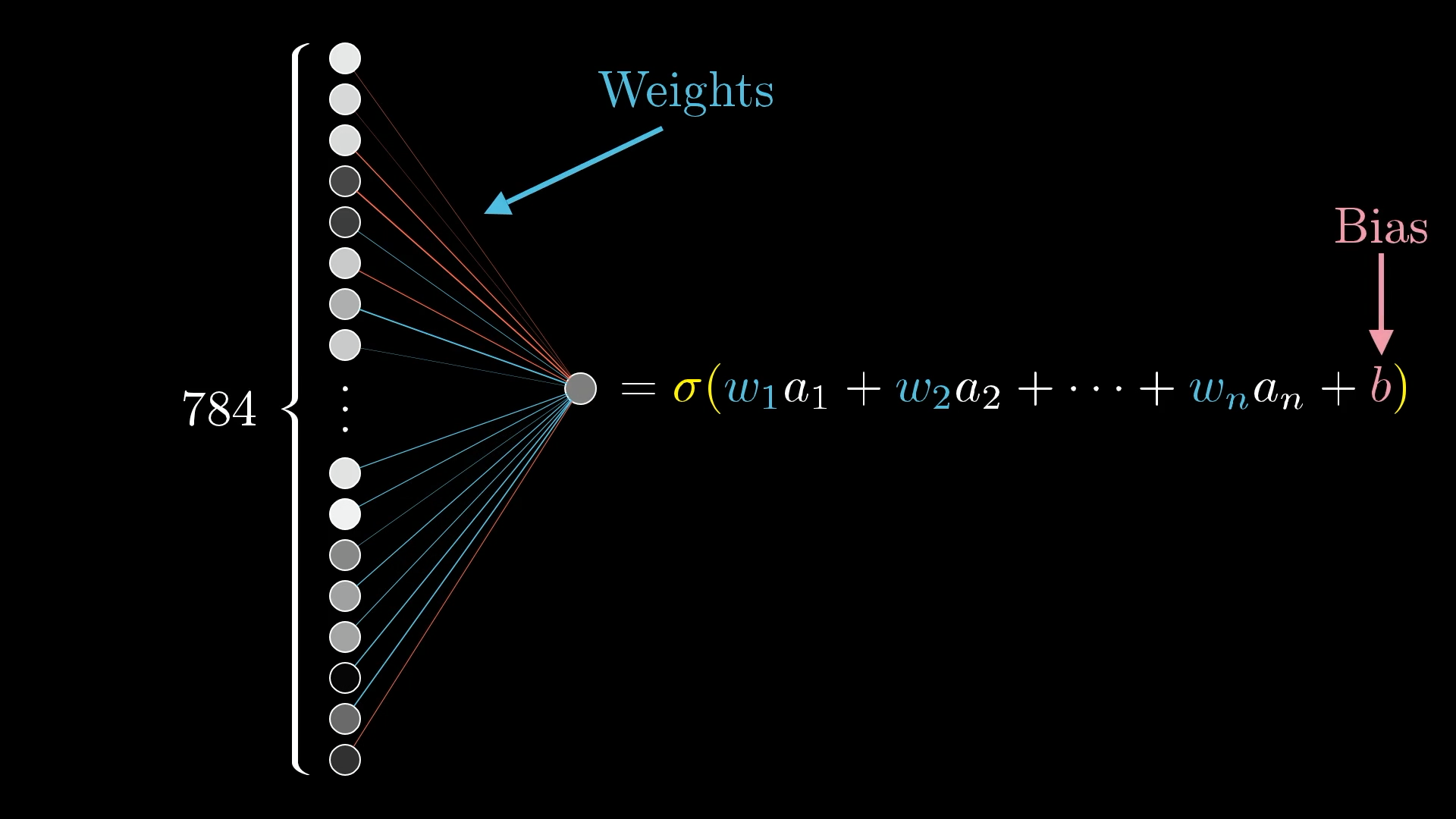
So, what we’re going to do is give each connection between our neuron and the ones in the first layer its own weight. You can just think of these weights as regular numbers that help decide how much influence each input has.
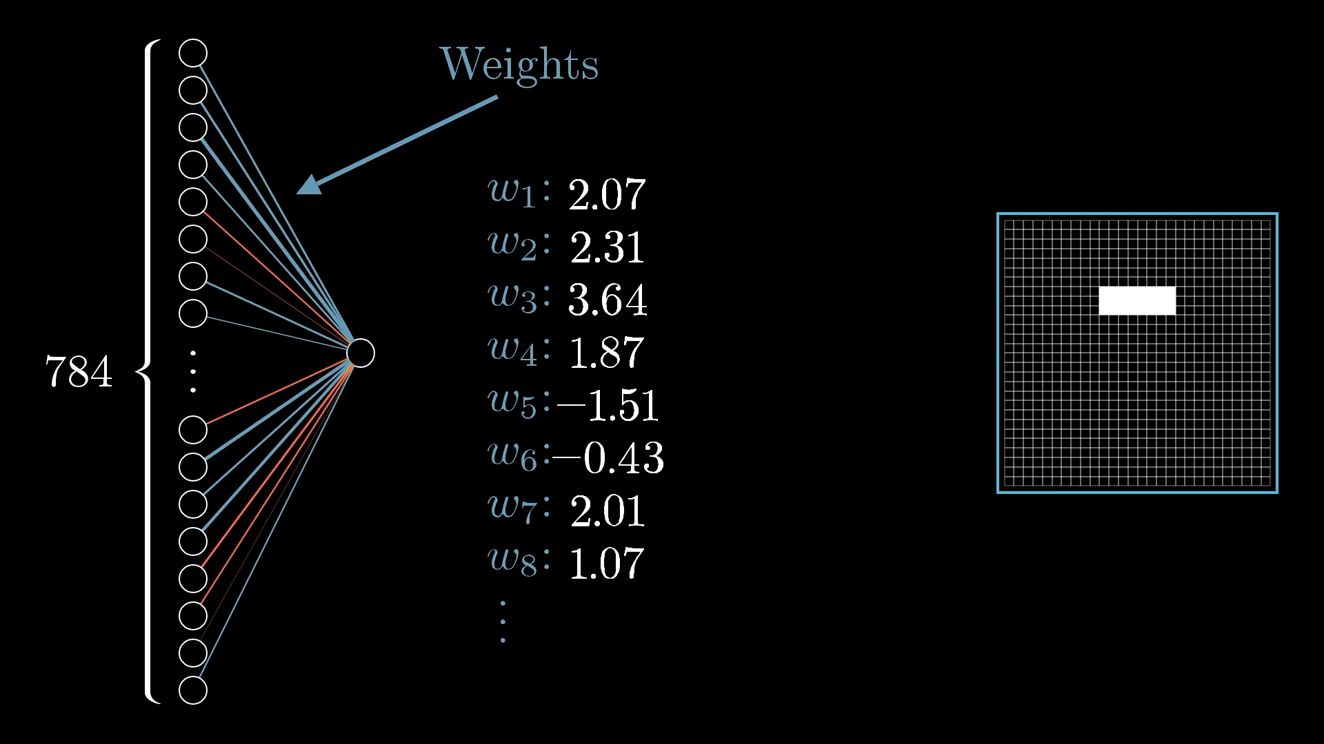
You can think of each weight as showing how much a neuron in the first layer influences this particular neuron in the second layer. If a neuron in the first layer is active, a positive weight means it encourages the second layer neuron to turn on too, while a negative weight means it tries to keep the second layer neuron off.
All these weights work together, sometimes helping and sometimes working against each other, but the idea is that when you add up all their effects, the neuron in the second layer will be pretty good at spotting the edge we want, as long as the weights are chosen well.
To figure out what the second layer neuron should do, you just take all the activations from the first layer, multiply each by its weight, and add them up.

It can be helpful to think of these weights as being organised into a grid of their own:
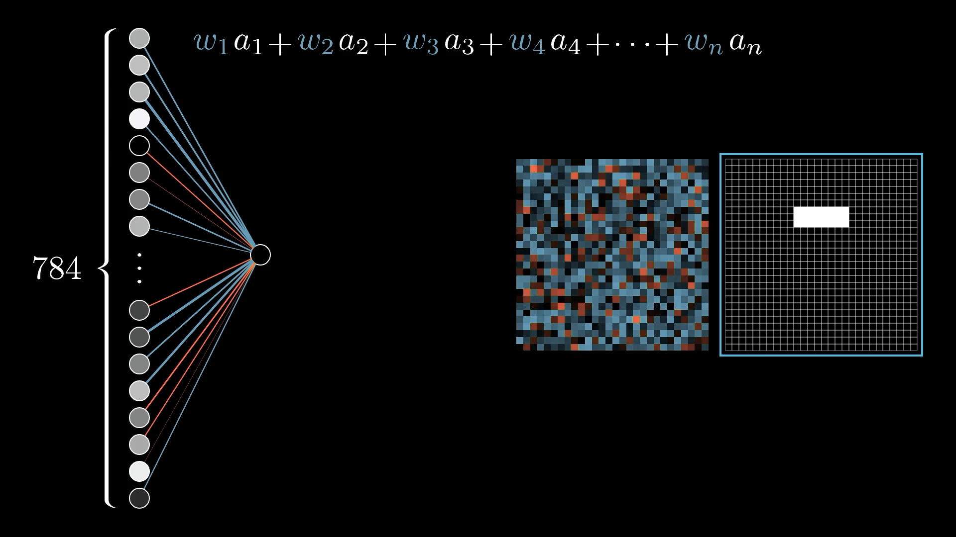
Blue pixels indicate a positive weight, and red pixels indicate a negative weight, with the brightness of that pixel being a depiction of the weight's value.
So what if we made the weights associated with almost all the pixels 0, except for some positive weights associated with these pixels in the region we want to detect an edge?
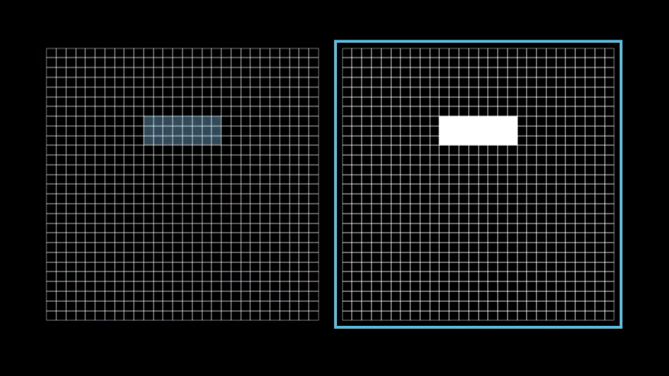
So, when you take the weighted sum of all the pixel values, what you’re really doing is just adding up the values of the pixels in the area you care about.
The thing is, if you set up your weights like this, you’ll end up detecting not just edges, but also any big bright blobs in that region. If you really want the neuron to focus on edges, it helps to add some negative weights around the area you’re interested in. That way, the sum gets highest when the pixels in the main region are bright, but the ones around it stay dark.
Sigmoid Squishification
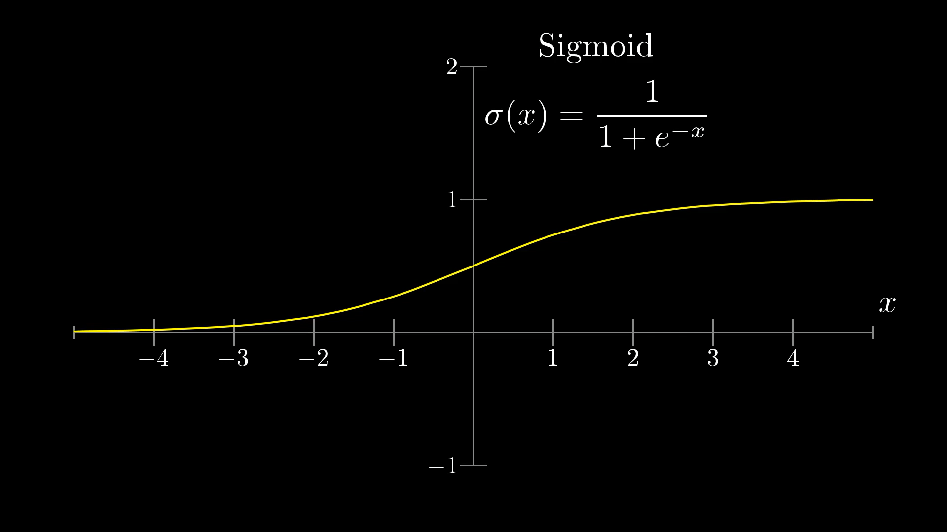
When you add everything up with the weighted sum, you can actually get any number at all, but for our network, we want the activations to always fall between 0 and 1. To make that happen, we usually run this sum through a special function that squeezes all possible numbers into that range.
A really popular choice for this is the "sigmoid" function, which is also called the logistic curve, and we use the symbol σ (sigma) for it. If you feed in a very negative number, the output will be close to 0, and if you give it a really positive number, it’ll be close to 1. In the middle, it smoothly transitions between those two, so the neuron's activation basically tells you how positive the weighted sum is.
But maybe we don’t actually want the neuron to turn on just because the weighted sum is a little above zero. Instead, we might want it to only become active when that sum gets pretty big, like above 10. In other words, we’d like to set things up so the neuron usually stays off unless there’s a strong enough signal, which is where the idea of a bias comes in.
To do this, we simply add a number, such as -10, to the weighted sum before we pass it through the sigmoid function, which squeezes everything into that nice range between 0 and 1.
We call this additional number a bias.
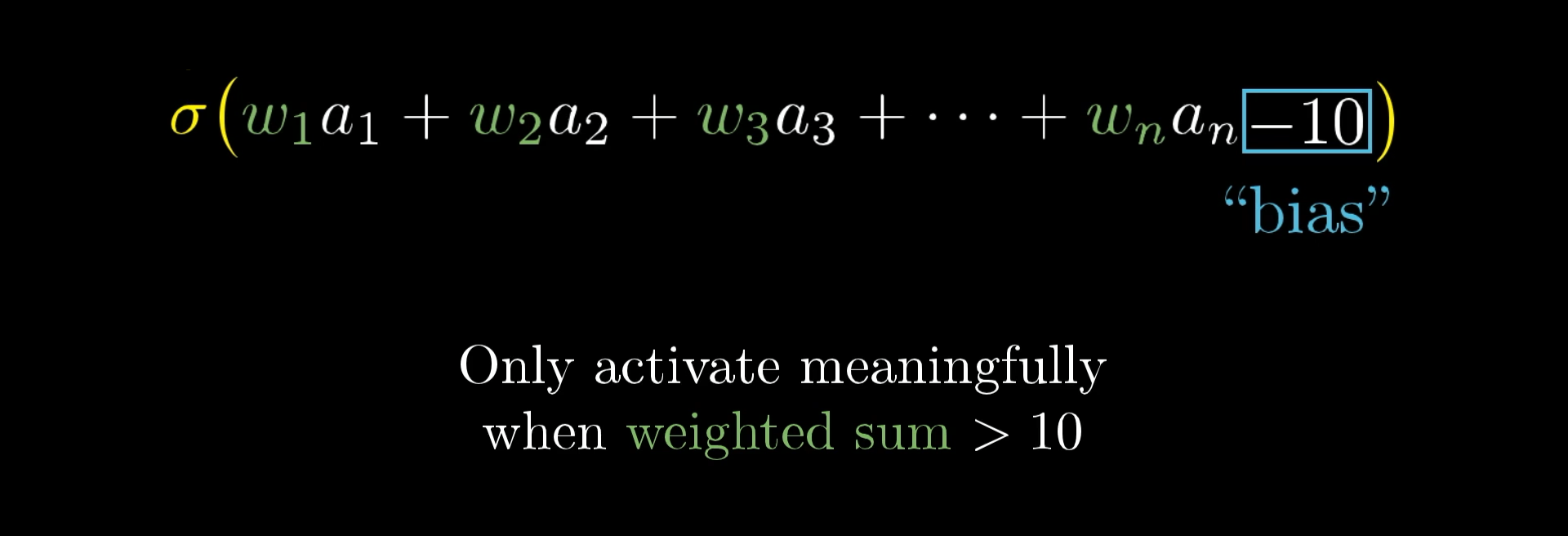
So the weights tell you what pixel pattern this neuron in the second layer is picking up on, and the bias tells you how big that weighted sum needs to be before the neuron gets meaningfully active.
More Neurons
And that’s just one neuron! Every single neuron in the second layer is connected to all 784 neurons from the first layer, each with its own weight. On top of that, each neuron gets its own bias, which is just another number added to the weighted sum before we run it through the sigmoid. It’s a lot to keep track of, right? For this hidden layer with 16 neurons, that means there are 784 times 16 weights, plus 16 biases.
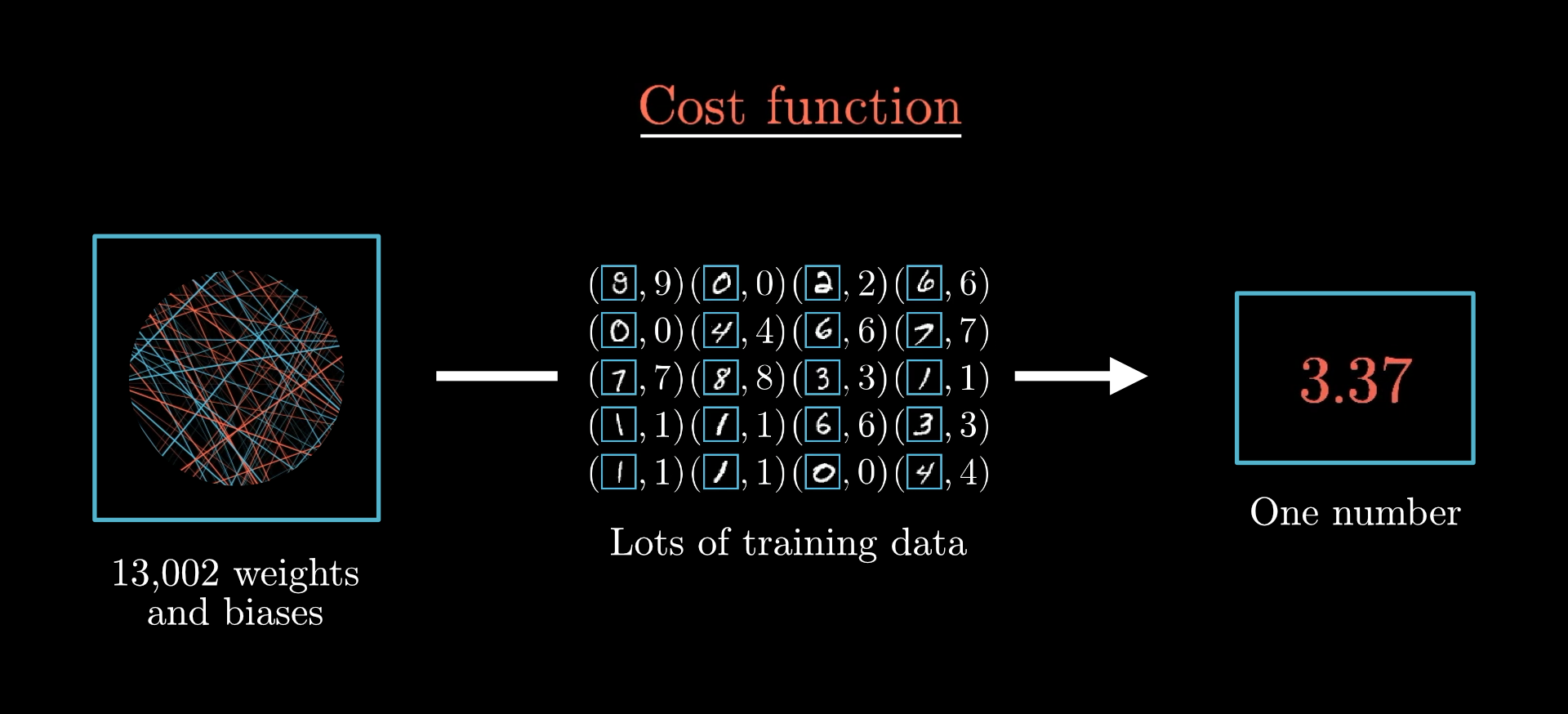
And remember, this is only for the connections between the first and second layers. The other layers have their own sets of weights and biases too. Altogether, this network ends up with 13,002 weights and biases in total. That’s 13,002 little knobs you can adjust to change how the network behaves.
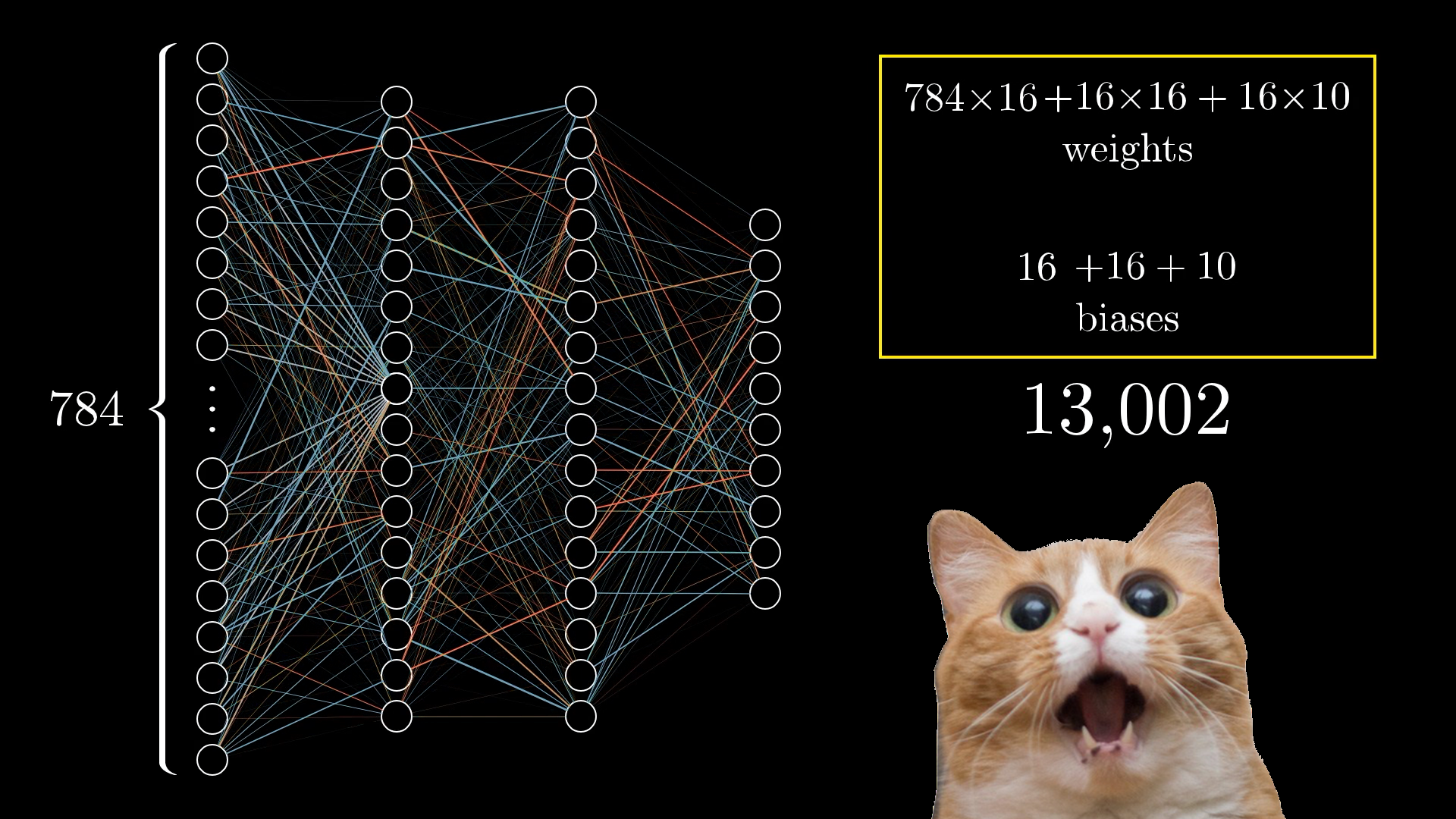
When we talk about learning in this context, we’re really just asking the computer to figure out the best possible values for all these different numbers, so it can actually solve the problem we care about.
Here’s a little thought experiment that’s both kind of amusing and a bit overwhelming, imagine trying to set every single weight and bias by hand. You’d have to decide exactly how to tweak things so the second layer notices edges, the third layer picks up on certain patterns, and so on.
Honestly, I find it pretty satisfying to think about what these weights and biases are actually doing, instead of just seeing the whole network as a mysterious black box. If the network isn’t behaving the way you expect, having some intuition about what these numbers mean gives you a place to start tinkering and improving things.
And even when the network does work, but maybe not for the reasons you thought, poking around in the weights and biases can really help you question your assumptions and see just how many different ways the network could be solving the problem.
More Compact Notation
Writing out the formula for how a single neuron gets its activation from the previous layer can get pretty messy and awkward.
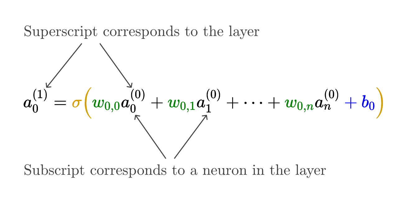
Keeping track of all those little indices is a pain, so let me show you a much tidier way to represent all these connections.
Rather than working out each weighted sum one at a time, we can use matrix multiplication to figure out all the activations for the next layer in one go.
To start, you just gather up all the activations from the first layer and stack them into a column vector.
Then, you arrange all the weights into a matrix, where each row matches up with all the connections from the first layer to a specific neuron in the next layer.
When you multiply the weight matrix by the activation vector, you get another column vector, and each entry in that vector is the weighted sum for a neuron in the next layer.
Instead of adding the bias to each value separately, we just collect all the biases into their own vector, and add that whole bias vector to the result of the matrix multiplication.
Finally, we apply the sigmoid function to every entry in that vector, so each neuron's activation gets squished into the range between 0 and 1.
Once you start using symbols for the weight matrix and these vectors, you can write out the whole process of moving from one layer’s activations to the next in a really compact and tidy way.
This approach makes the code way cleaner and a lot faster, since most libraries are really good at matrix multiplication.
Just as a quick aside, because machine learning and neural networks have gotten so popular, there’s been a ton of progress in special hardware that can do matrix multiplication super quickly. For example, Google’s “Tensor Processing Unit,” or TPU, is built for this kind of thing.
Honestly, when you hear about some new “neural architecture” that’s supposed to be a big leap for AI, a lot of the time, what’s really going on is that they’ve found a way to multiply matrices even faster.
To be fair, this hardware can do more than just matrix multiplication, but that’s the main thing that sets it apart. And if you get what we just talked about, you’ll see why that matters.
The Network Is Just a Function
Earlier, I mentioned that you can think of these neurons as just “things that hold numbers.” But really, the number each neuron holds changes depending on the image you give the network. So, it’s actually more accurate to picture each neuron as a little function. It takes in all the activations from the previous layer and gives you back a number between 0 and 1.
If you zoom out, the whole network itself is just one big function. You feed in 784 numbers (which come from the image’s pixels), and out come 10 numbers (one for each possible digit). Sure, it’s a wildly complicated function, since it’s got over 13,000 parameters (all those weights and biases), and it’s made up of lots of matrix multiplications and sigmoid squishing steps. But at the end of the day, it’s still just a function.
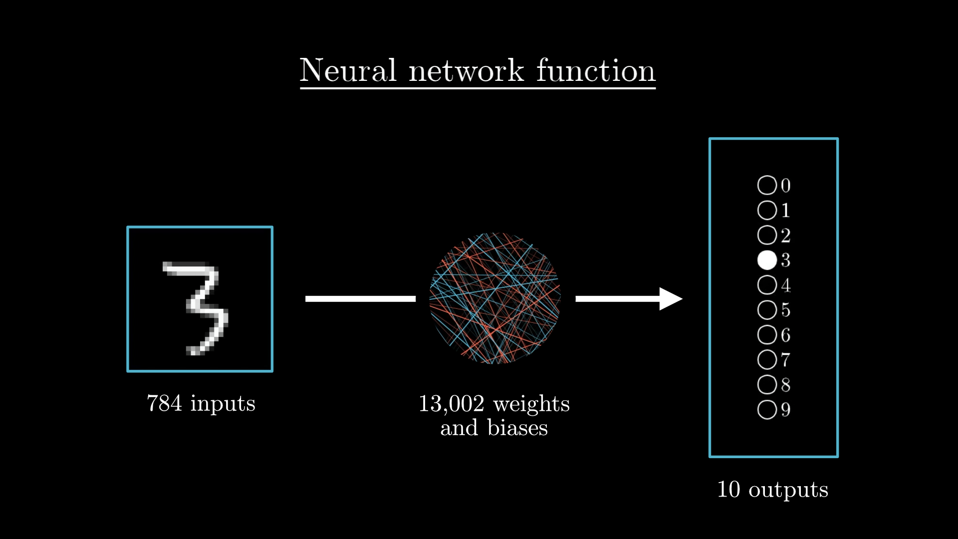
Honestly, it’s kind of comforting that the network looks so complex. If it were much simpler, it probably wouldn’t stand a chance at figuring out something as tricky as recognising handwritten digits.
But that brings up a big question of how does the network actually learn the right weights and biases from the data in the first place?
How the Network Learns
What really sets machine learning apart from traditional computer science is that you don’t spell out step-by-step instructions for the task you want to solve. For example, you never actually write out a set of rules for recognising digits. Instead, you build a system that can look at lots of example images of handwritten digits, each one labelled with the correct answer, and then it tweaks its 13,002 weights and biases to get better at making the right guesses.
All those labelled images we give to the network are called the “training data”.
The hope is that, thanks to the way the network is structured, it will pick up on patterns that help it do well not just on the training data, but also on new images it hasn’t seen before. To check if that’s happening, we test the network after training by giving it more labelled images it hasn’t seen and seeing how well it does at classifying them.
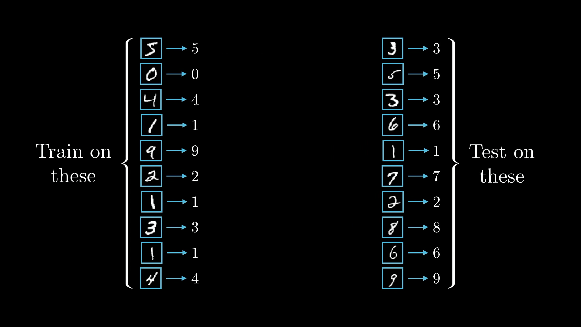
This whole process needs a lot of data. Luckily, the people behind the MNIST database have put together tens of thousands of handwritten digit images, each one labelled with the correct number, and they’ve made it available for anyone to use.
I should point out that although it can be easy to describe a machine as "learning", once you see how it works, it feels a lot less like some crazy sci-fi premise and a lot more like a calculus exercise. It really just comes down to finding the minimum of a specific function.
The Cost Function
Just to recap, everything the network does depends on its weights and biases. The weights basically tell you how strong the connections are between neurons in one layer and the next, while each bias kind of nudges its neuron to be more likely to fire or stay quiet.
When you first set up the network, you just pick random numbers for all the weights and biases. At this point, the network is going to do a terrible job on any training example, because it’s just guessing.
Like, if you give it a picture of a 3, the output you get is just a jumble of numbers that doesn’t make any sense:
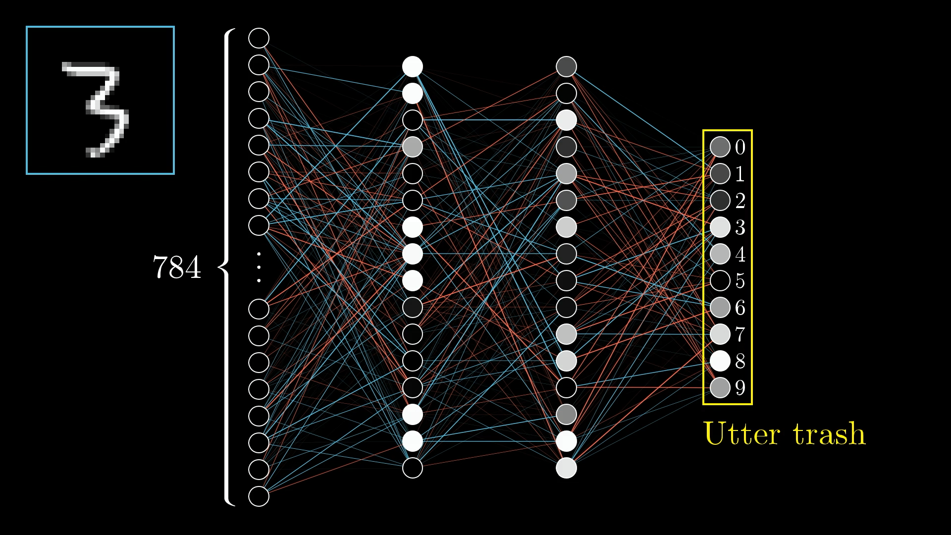
So, how do you actually tell if the computer is getting things wrong, and how do you help it get better?
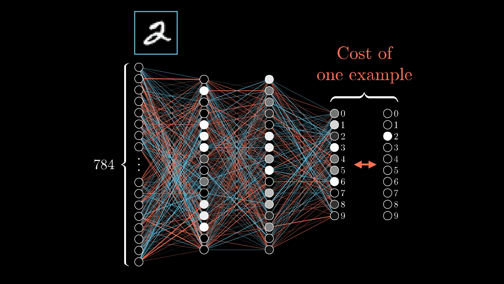
So, the next step is to set up something called a cost function. This is basically a way to let the computer know, “Hey, that output isn’t what we’re looking for. Most of those neurons should be at zero, except for the one that matches the correct answer, which should be at one. What you just gave me is way off.”
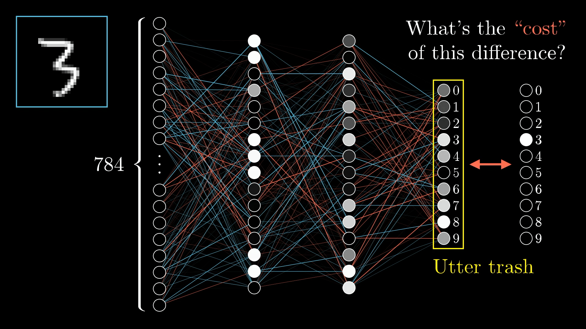
If you want to put it in more mathematical terms, you just take the difference between what the network actually spits out and what you want it to say, square those differences for each output, and then add them all up. That total is what we call the “cost” for that particular training example.
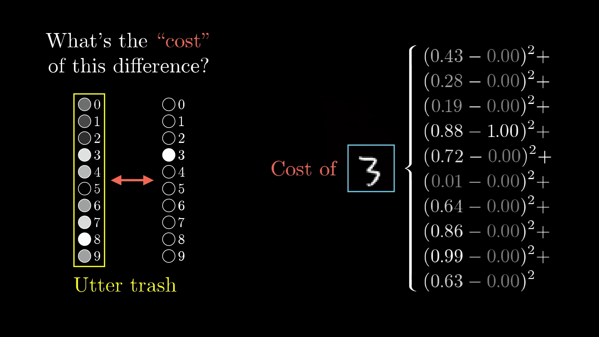
The idea is that the cost will be low when the network gets the answer right with confidence, and it’ll be high when the network is confused or just plain wrong.
The Cost Over Many Examples
But we don’t just care about how the network does on a single image. To really see how well it’s working, we have to look at the average cost across all those tens of thousands of training images. That average basically tells us how much the network is struggling overall, or how much room there is for improvement.
Now, this isn’t a simple thing to calculate. Just as a reminder, the network itself is already a pretty complex function, with 784 inputs (those are the pixel values), 10 outputs, and 13,002 parameters.
The cost function adds another layer of complexity on top. Instead of taking in images, it takes all 13,002 weights and biases as its input, and then gives you a single number that sums up how well (or badly) those weights and biases are doing. It’s all based on how the network performs across the entire training set, so you can think of the training data as a huge part of what shapes this cost function.
Minimising the Cost Function
Just telling the computer it’s doing a bad job isn’t enough. What we really want is to guide it, to show it exactly how to tweak those 13,002 weights and biases so it can actually get better.
We can do better! Growth mindset!

To make things a bit simpler, instead of wrestling with a cost function that has 13,002 different inputs, let’s just imagine a much easier case: a function that takes in one number and spits out one number.
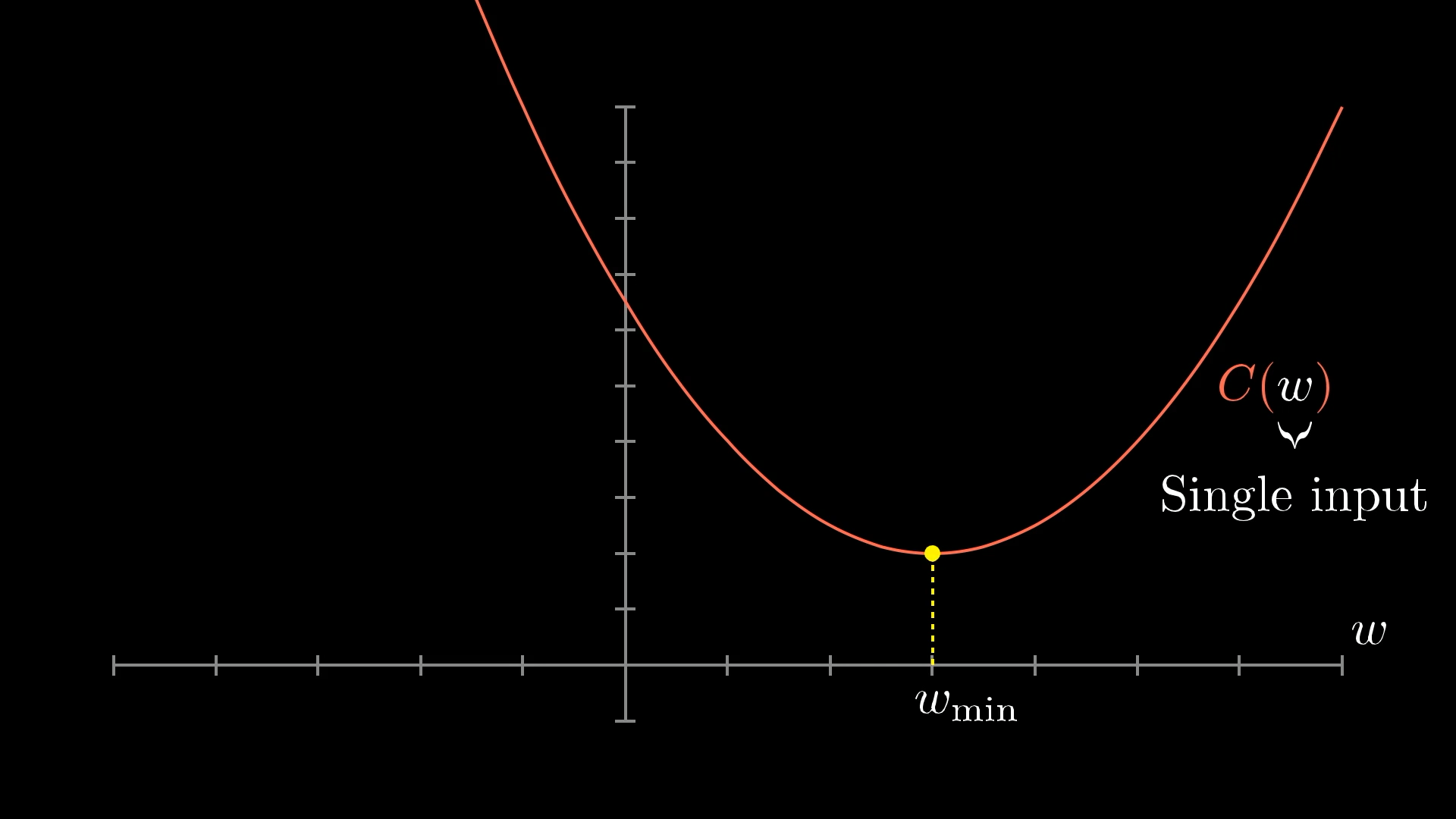
So, how do you actually find the input that makes this cost function as small as possible?
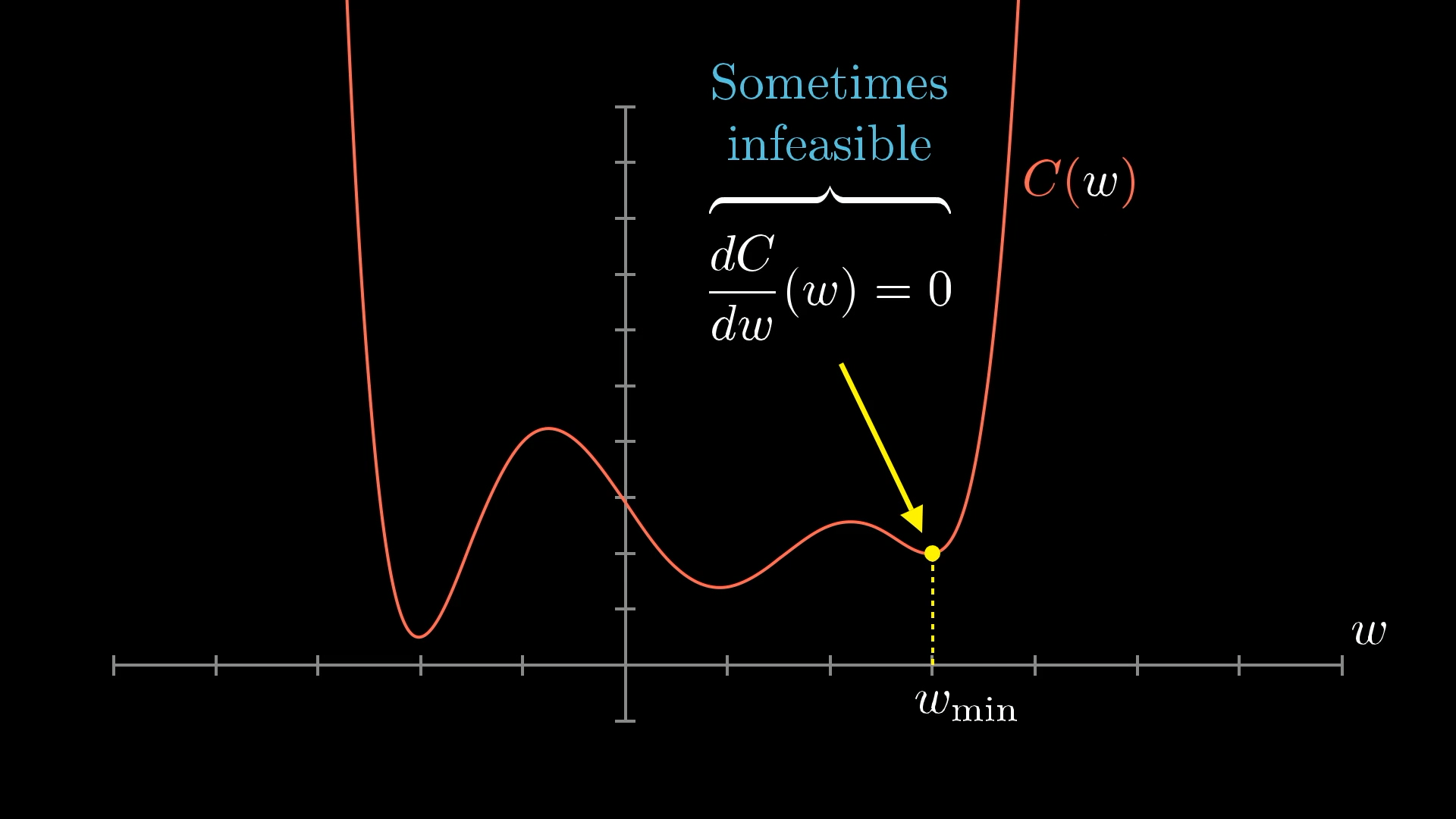
If you’ve done some calculus before, you might know that sometimes you can find the minimum by setting the slope to zero and solving for it. But for really complicated functions, that’s just not practical, and for our giant 13,002 input function, it’s definitely not going to work.
A much more practical approach is to just pick a random starting point and then figure out which way to move to make the output smaller. Basically, you check the slope of the function where you are. If the slope is negative, you move to the right. If it’s positive, you move to the left.
You keep checking the slope and taking little steps in the right direction, and over time, you’ll get closer and closer to a low point in the function.
The best way to picture this is to imagine a ball rolling down a hill:
Even with this simple cost function that only takes one input, you can end up in all sorts of different valleys depending on where you start. Basically, if you pick a random starting point, you might not always find the lowest possible spot, just a low spot nearby, and there’s no promise it’s the very best one.
Another thing to notice is that if you make your steps depend on how steep the slope is, your steps naturally get smaller as you get closer to the bottom. When the slope flattens out near a minimum, you’ll take tinier and tinier steps, which helps you avoid jumping past the lowest point.
Now, let’s make things a little more interesting. Imagine a function that takes two inputs instead of one. You can picture the input space as a flat plane, like an xy-grid, and the cost function forms a kind of landscape or surface above it.
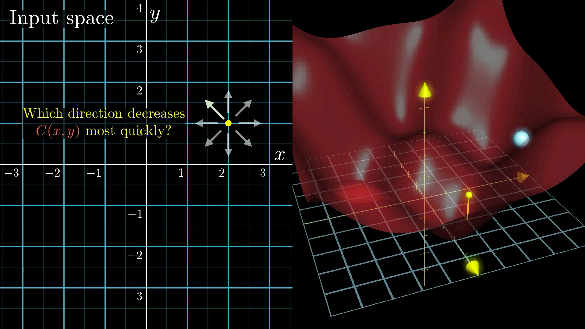
Instead of just thinking about the slope in one direction, you’re now figuring out which way to move in this plane to make the cost drop the fastest. It’s still like a ball rolling down a hill, just in a more complex landscape.
Beyond Slope: Using the Gradient
When you’re working in higher dimensions, talking about the “slope” as just a single number doesn’t really make sense anymore. Instead, you need a whole vector to show you which way is the steepest uphill.
If you’ve done a bit of multivariable calculus, you might recognise this as the “gradient”. The gradient points in the direction where the function increases the fastest, so if you want to make the function bigger, you’d step that way.
But since we want to make our cost function smaller, we actually want to go in the opposite direction, so we take the negative of the gradient. The length of this gradient vector also tells us how steep things are at that spot.
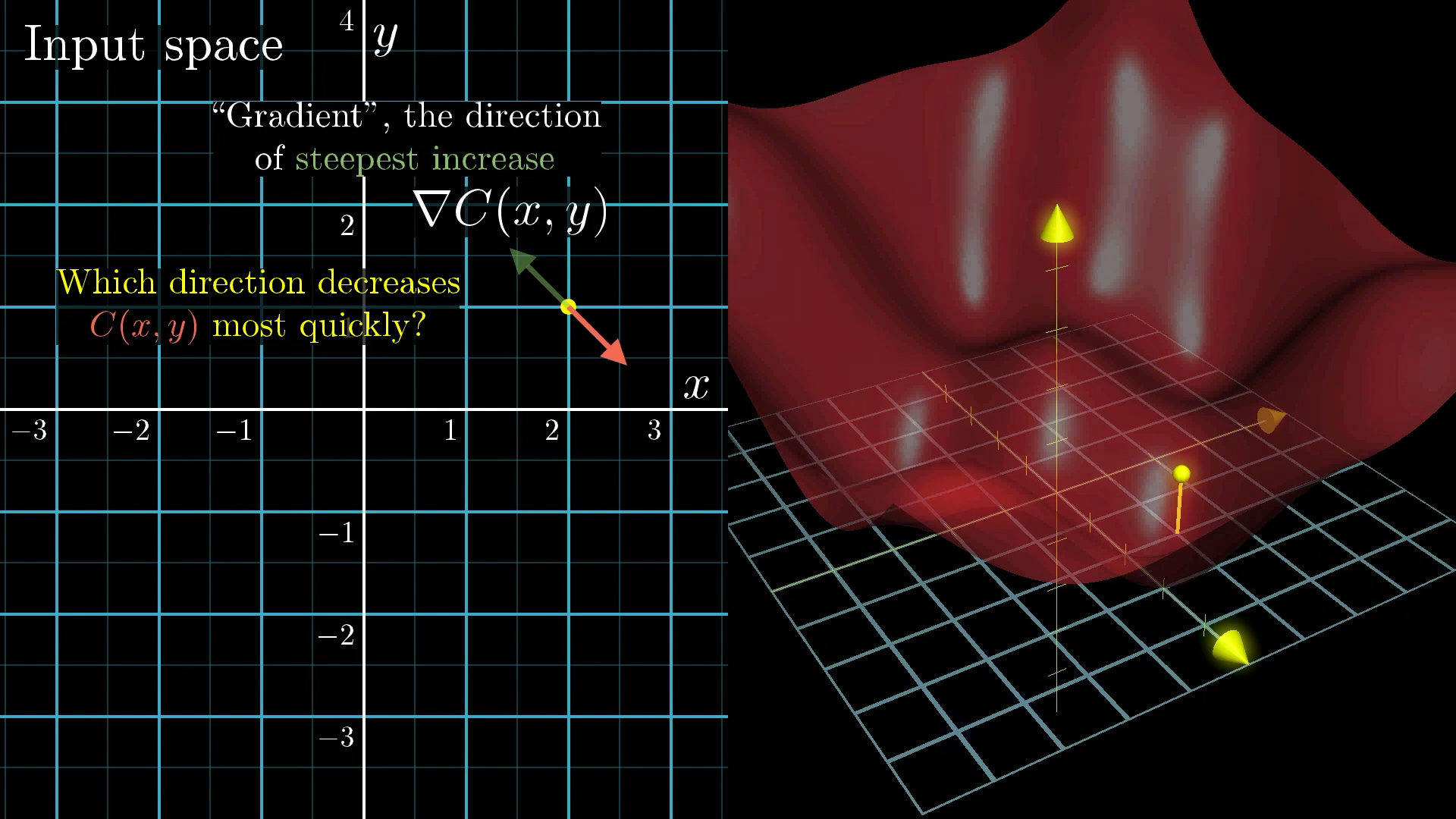
So, the basic idea for finding the minimum is to figure out the gradient, take a step downhill, and keep repeating that. This whole process is called “gradient descent”.
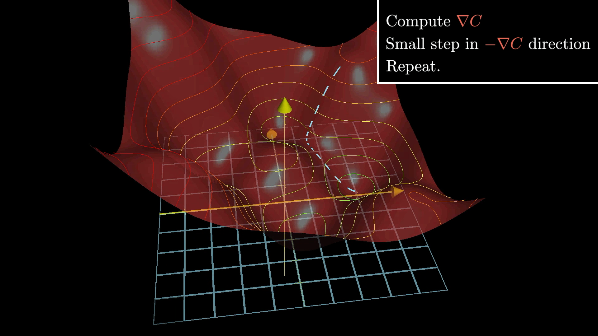
Just to remind you, our cost function is built to measure how badly the network is doing on the training data. So, if we keep adjusting the weights and biases to make the cost go down, the network should get better at its job.
When you actually do this in practice, each step looks like −η∇C, where η (eta) is the learning rate. If you make η bigger, your steps get bigger, so you might reach the minimum faster, but you also risk overshooting and bouncing around too much.
This whole idea works the same way even if your function has 13,002 inputs instead of just two. I’m still showing the two input version because it’s way easier to picture, but in reality, we’re just nudging things around in a space that’s way too big to imagine. I’ll try to explain it in a way that doesn’t need a picture now.
Another Way to Think About The Gradient
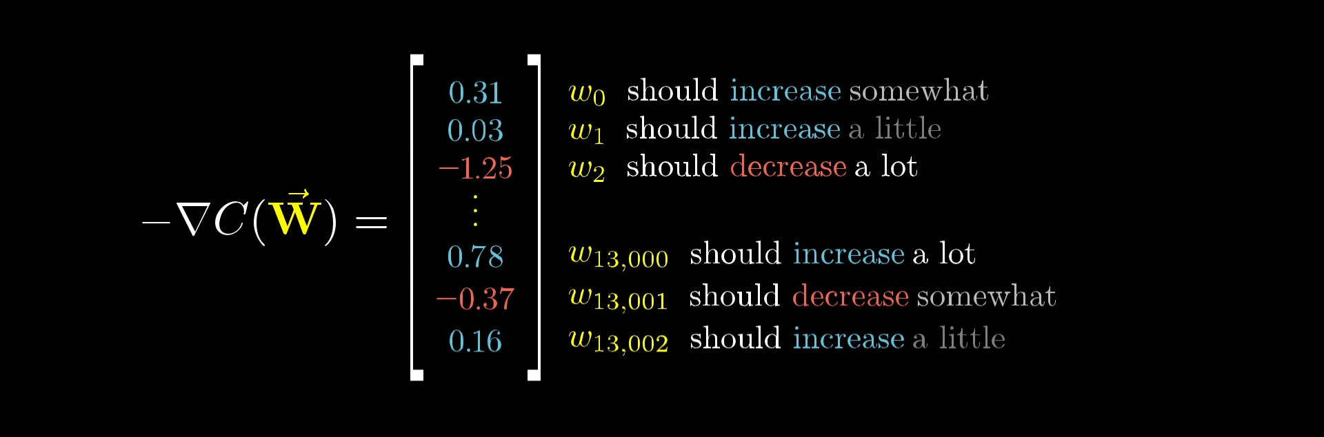
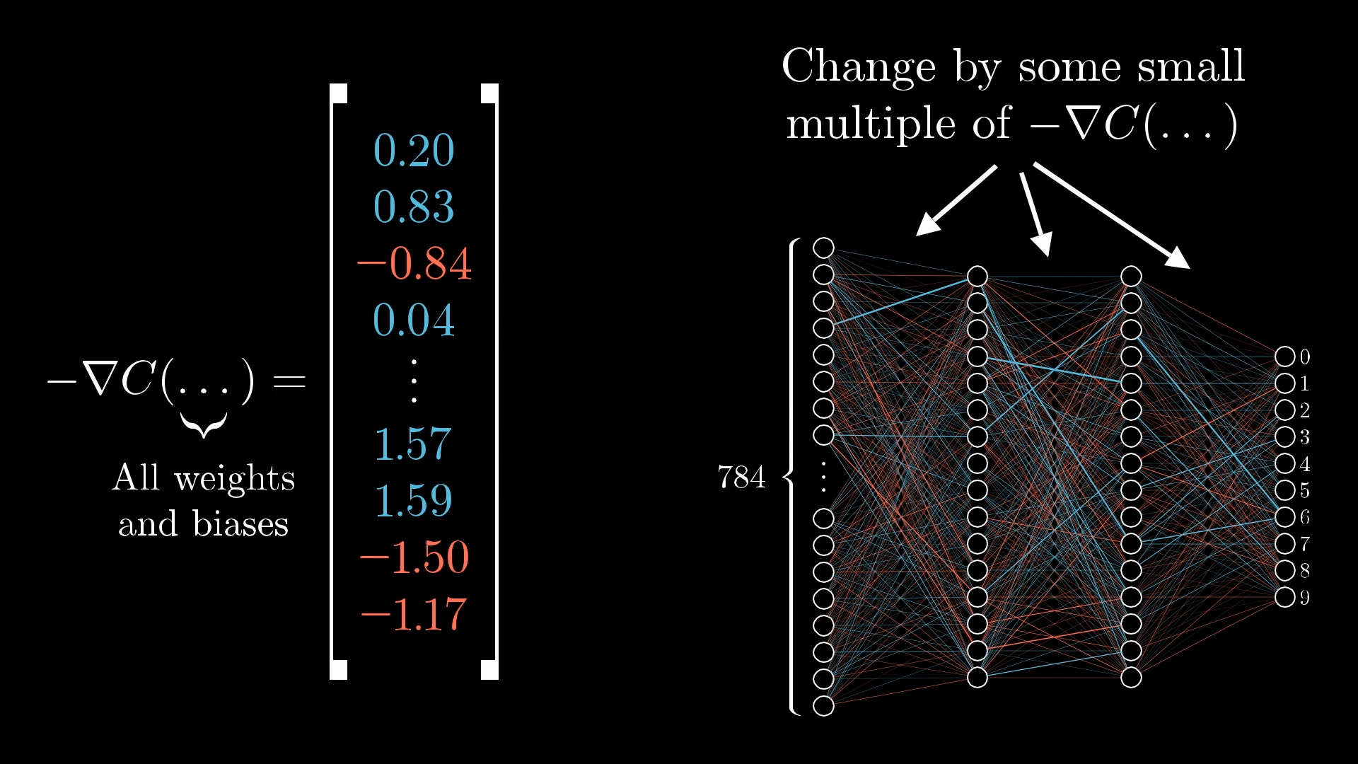
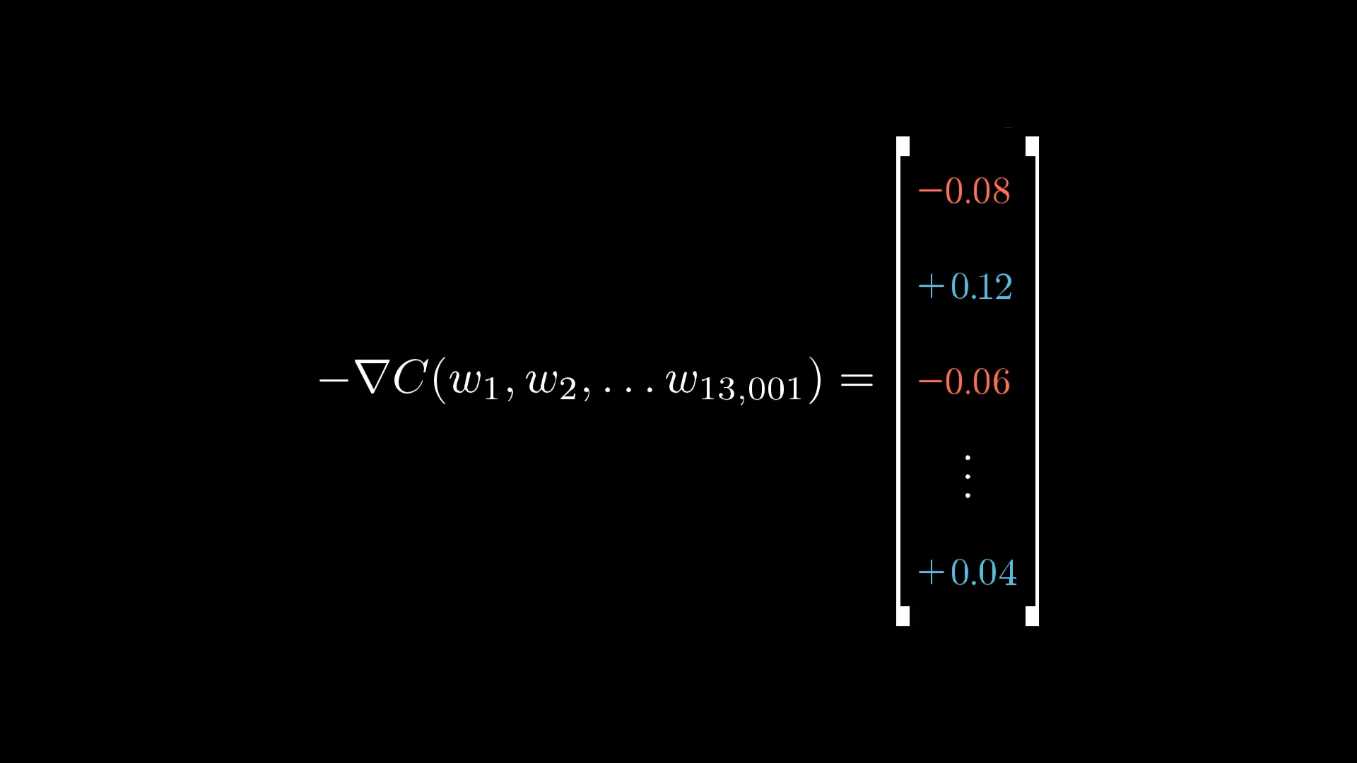
Let’s try to picture all the weights and biases in the whole network as one giant column of numbers, there are 13,002 of them in total. Now, the negative gradient of the cost function is just another column with 13,002 numbers, one for each weight and bias.
The column on the left is every single weight and bias in the network, and the column on the right is the negative gradient. That negative gradient is basically a list of tiny adjustments you should make to each weight and bias if you want to move in the direction that lowers the cost the fastest.
This negative gradient points you in the best direction to tweak all 13,002 numbers at once, so the cost function drops as quickly as possible.
Each part of the negative gradient tells you two things: first, the sign tells you whether to nudge that particular weight or bias up or down, and second, the size tells you how important that nudge is compared to the others.
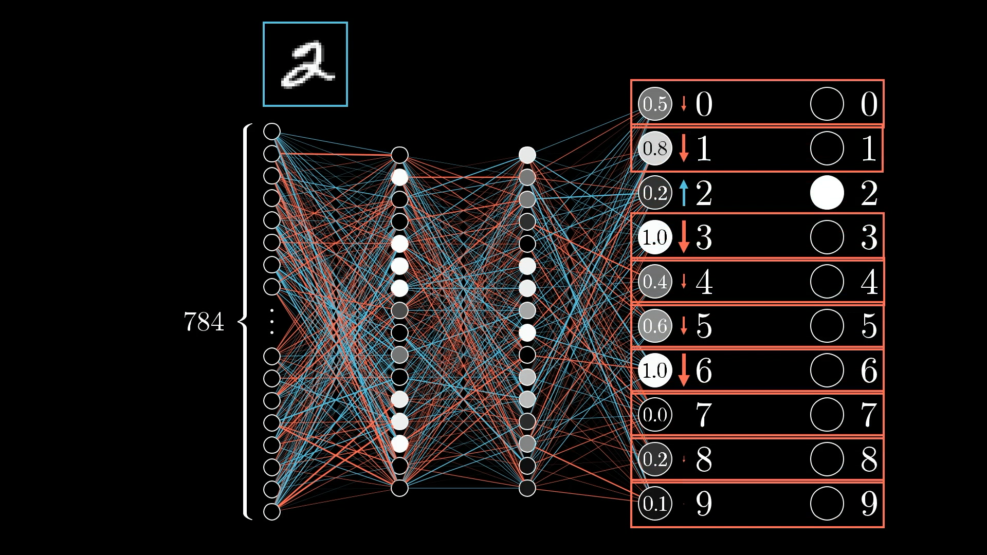
In our network, changing one weight might make a much bigger difference to the cost than changing another. For example, take a look at the image below and imagine the network is trying to decide if the input is a 3.
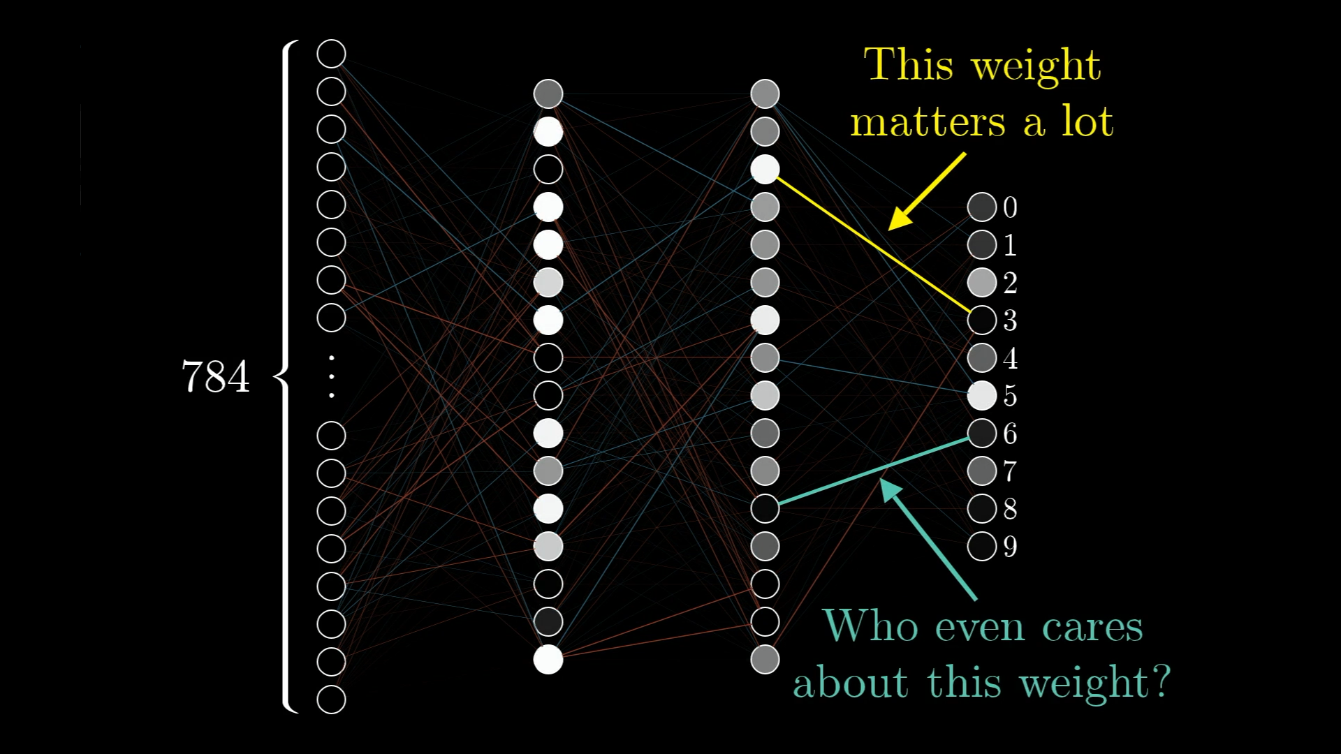
Some connections are just more important for getting the right answer on our training data. You can think of the gradient as a way of showing which weights and biases matter most, basically, which tweaks will give you the most improvement for your effort.
So, if the cost function adds a layer of complexity on top of the neural network, the gradient adds another layer, showing you exactly how to adjust everything to make the cost drop as quickly as possible.
The method we use to actually figure out this gradient efficiently is called backpropagation, and that’s what we’ll look at next. I want to really break down what happens to each weight and bias for a single piece of training data, so you get a feel for what’s going on behind all the formulas.
The main takeaway here, no matter how it’s implemented, is that when we say a network is “learning,” we’re really just talking about changing the weights and biases to make the cost function smaller, which means the network gets better at its job on the training data.
What is Backpropagation?
Alright, so the negative gradient of the cost function is really just a giant vector with 13,002 numbers in it, and each one tells us how to tweak a specific weight or bias to make the cost go down as efficiently as possible. Backpropagation is just the method we use to actually figure out what this negative gradient is.
Now, trying to picture a vector in 13,002 dimensions is pretty much impossible for any of us, so don’t worry if that sounds wild.
Instead, it helps to think about what each number in that vector means. The size of each part of the gradient tells you how much the cost function reacts to changes in that particular weight or bias.
For example, let’s say you run the backpropagation process and get a negative gradient where one weight has a value of 3.2, and another has just 0.1:
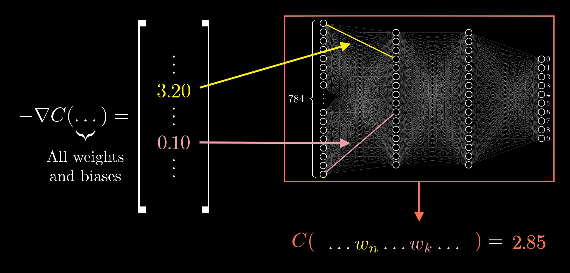
What this means is that the cost function is 32 times more sensitive to changes in that first weight than the second one. So, if you nudge the first weight a little, you’ll see a much bigger effect on the cost than if you nudge the second one by the same amount.
The Intuition for Backpropagation
When I first started learning about backpropagation, what really tripped me up was all the complicated notation and trying to keep track of the different indices.
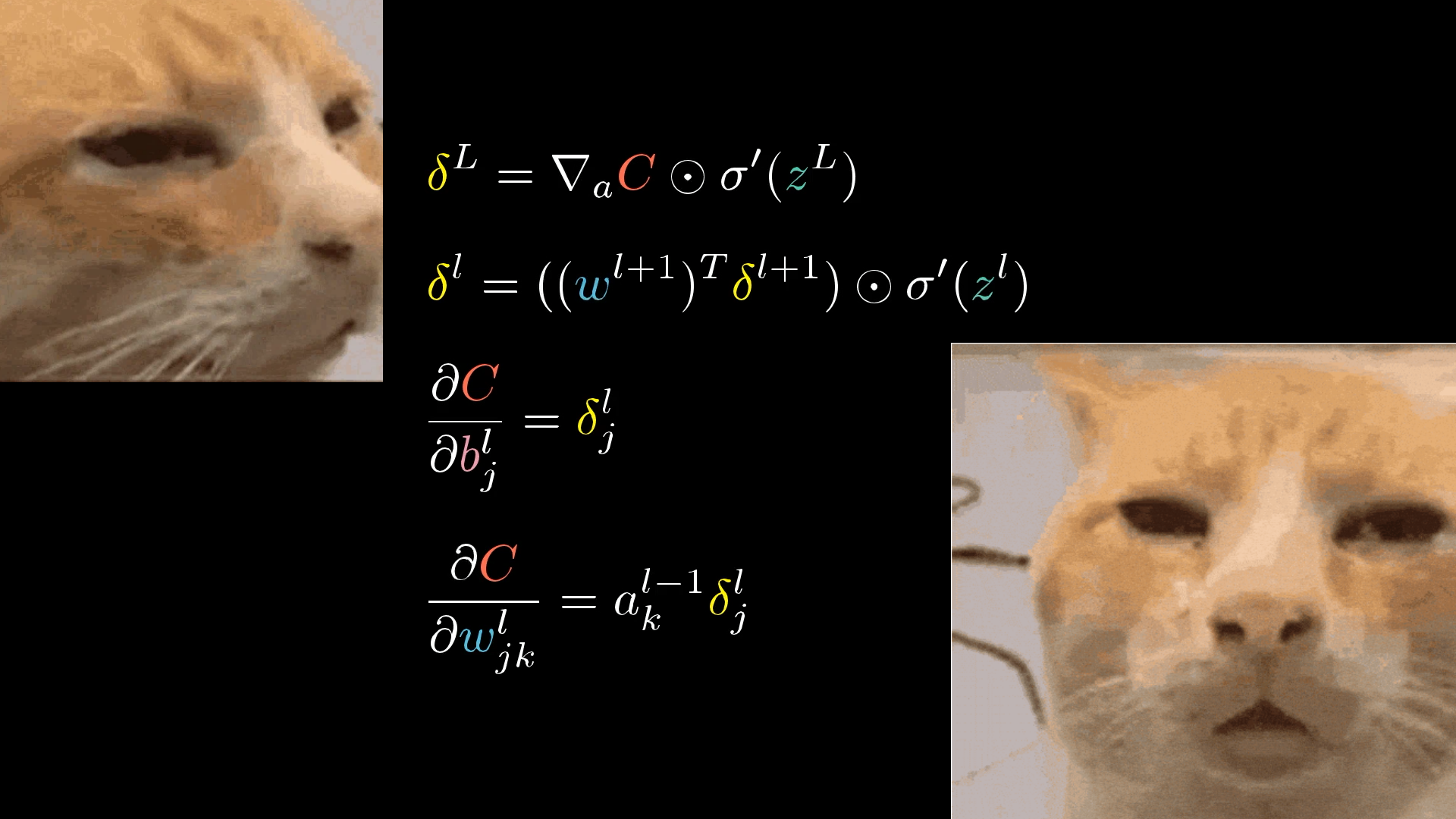
There’s just so much notation thrown around, and it can feel overwhelming. What does it all even mean?
For this blog post, let’s not worry about the notation at all. Instead, I want to walk you through what actually happens to the weights and biases when we look at each training example.
The full cost function is calculated by averaging the cost for each example across tens of thousands of training images, so when we update the weights and biases during a single step of gradient descent, it technically depends on every single example. In practice, though, we’ll use a little trick later on to avoid having to process every single example for every update, which makes things much more efficient.
But for now, let’s just zoom in on one example, say, this image of a 2:
What does this one training example actually do to the way we should adjust the weights and biases?
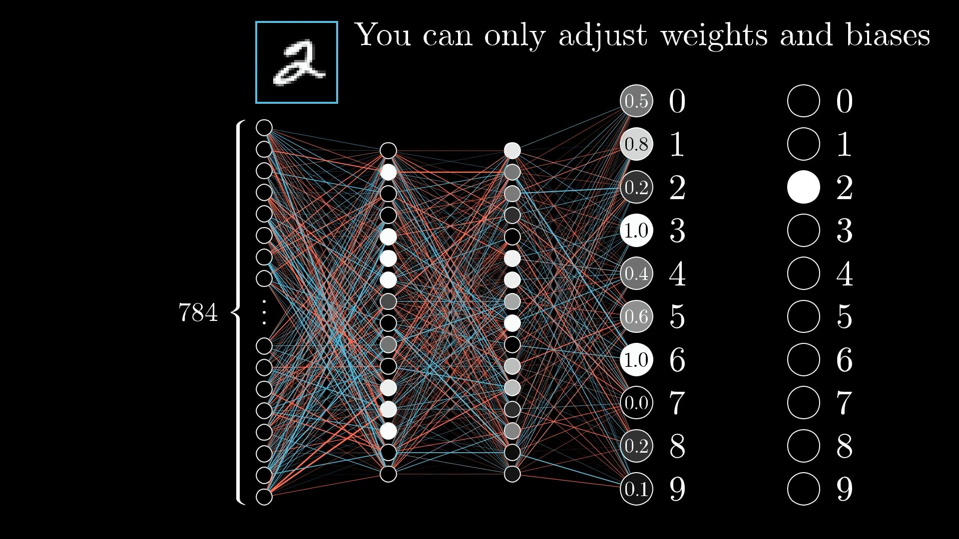
Since the network isn’t trained yet, the activations in the output layer are basically random. That’s not what we want, we want those activations to clearly point to the digit 2.
But here’s the thing: we can’t directly change the activations themselves. The only things we can actually tweak are the weights and biases, so we need to figure out how to nudge those in a way that gets the output closer to what we want.
Even though we can’t just set the activations to what we want, it’s still useful to keep track of the changes we wish we could make in that output layer, and then work backwards to see how to adjust the weights and biases to make that happen.
Because we want the network to recognise this as a 2, our goal is to boost the value of the neuron for digit 2, while nudging the values for all the other digits down:
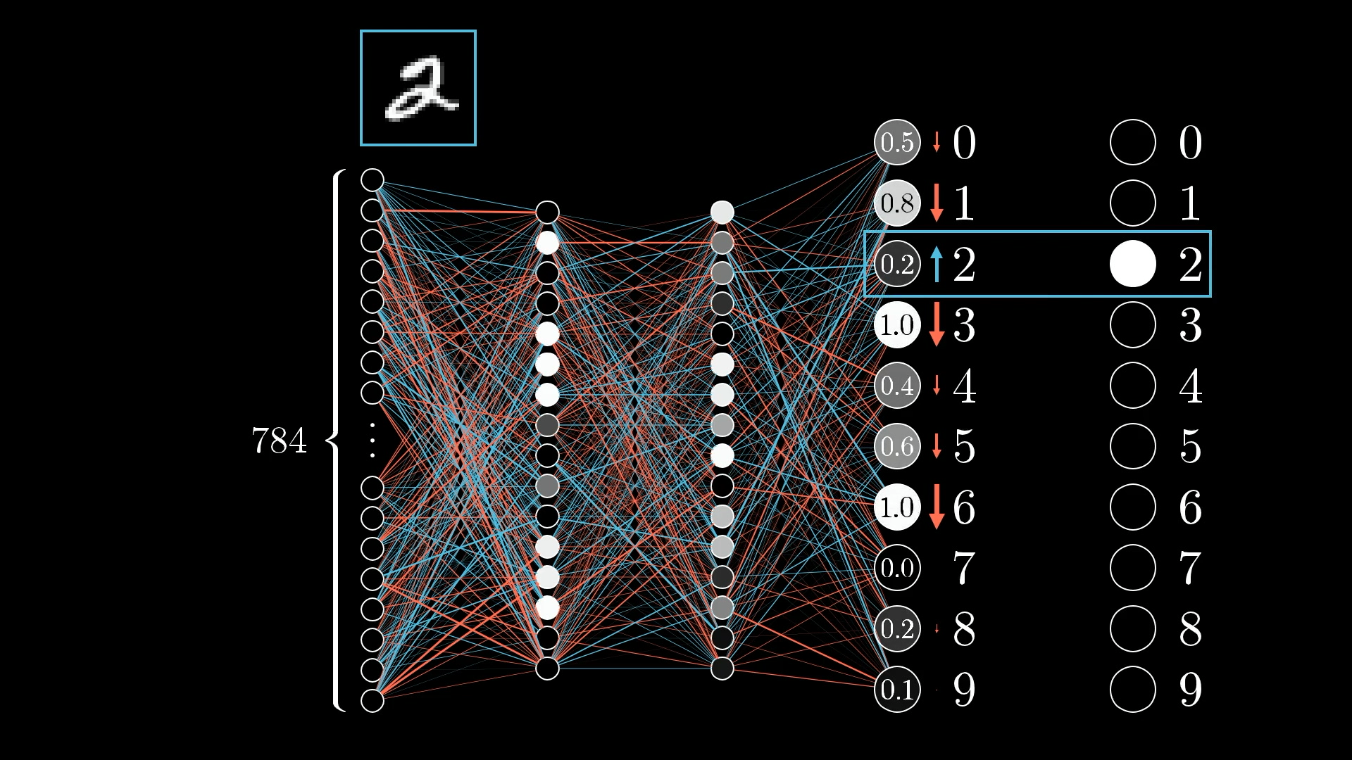
And the amount we nudge each one really depends on how far off it is from what we want. If a neuron's output is way off, it needs a bigger adjustment, but if it's already pretty close, just a small tweak will do.
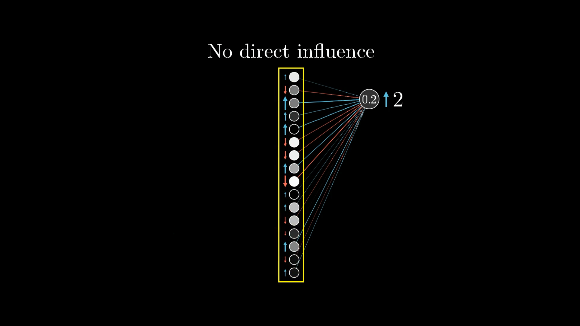
Let’s zoom in on the neuron for the digit 2, since that’s the one we want to push higher:
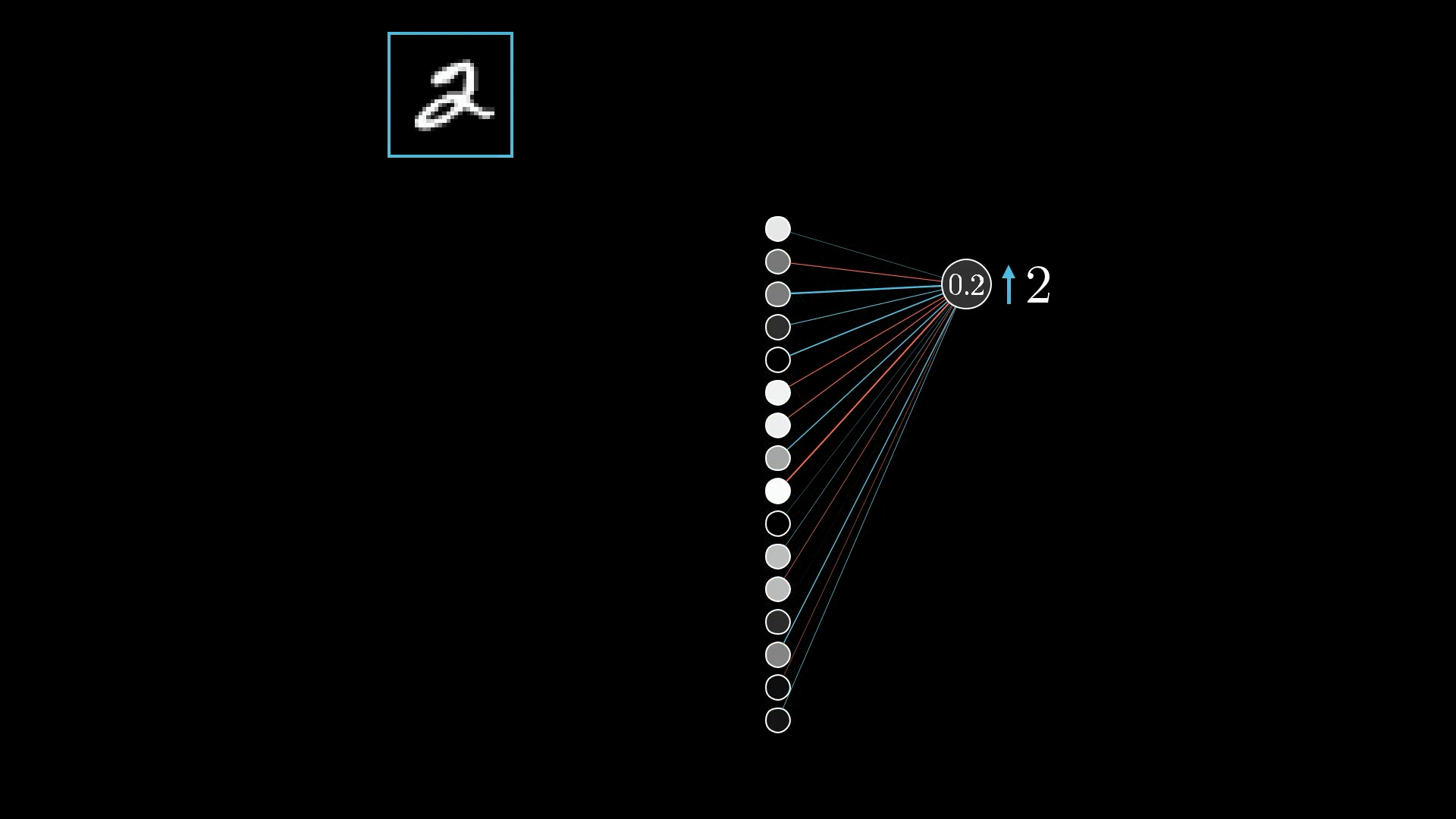
The activation for this neuron (like 0.2 in this example) comes from adding up all the activations from the previous layer, each multiplied by its own weight, then adding a bias, and finally running that total through something like the sigmoid function to squish it between 0 and 1:
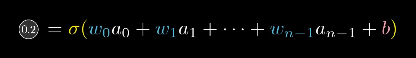
So, there are three main ways that can work together to bump up this activation:
- Increase the bias
- Increase the weights
- Change the activations from the previous layer
Changing the Bias
Changing the bias associated with a neuron is the simplest way to change its activation. Unlike changing the weights or the activations from the previous layer, the effect of a change to the bias on the weighted sum is constant and predictable.
Changing the Weights
So, how do we actually go about tweaking the weights? Well, since each weight gets multiplied by the activation from the previous layer, not all weights have the same impact. The ones connected to the brightest, most active neurons matter the most, because their activations are bigger, so any change to those weights will have a bigger effect on the output.
If you boost a weight that's linked to a really active neuron, you'll see a bigger change in the cost function than if you tweak a weight that's connected to a less active (dimmer) neuron. Of course, we're just talking about the effect for this one training example right now.
When we're using gradient descent, it's not just about whether to increase or decrease each weight, it's about figuring out which changes will make the biggest difference for the least effort.
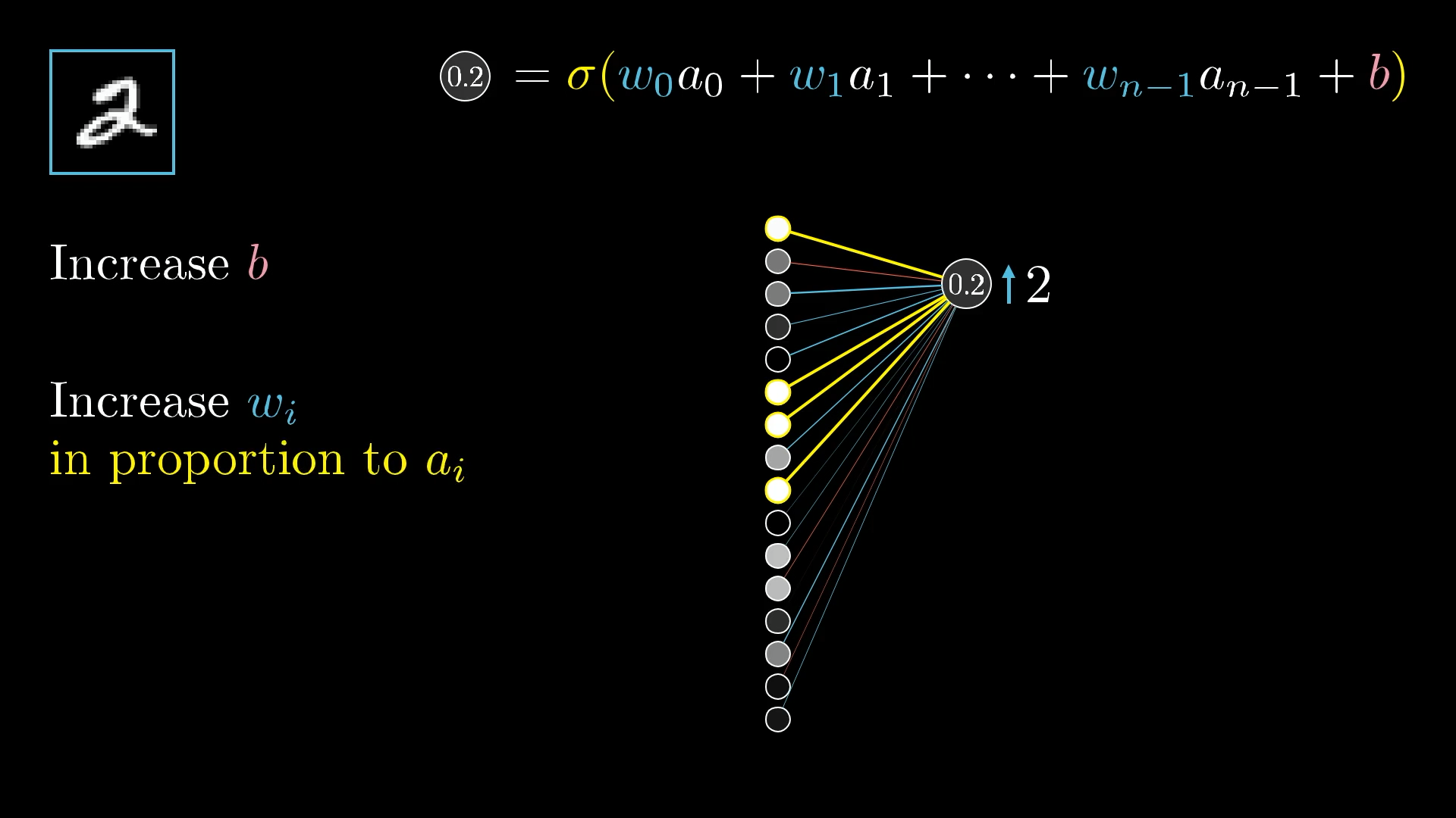
So, to get the most out of your updates, you want to adjust each weight in proportion to how active its associated neuron is.
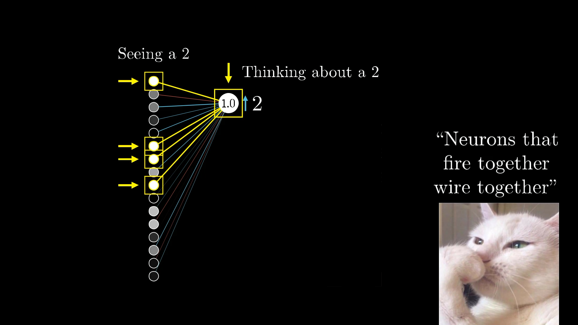
Interestingly, this idea is kind of similar to something in neuroscience called Hebbian theory, which is often summed up as "neurons that fire together wire together." In our case, the strongest connections (the biggest increases in weights) happen between the neurons that are most active and the ones we want to become more active.
Basically, the neurons that light up when the network sees a 2 end up getting more strongly connected to the ones that represent the idea of a 2.
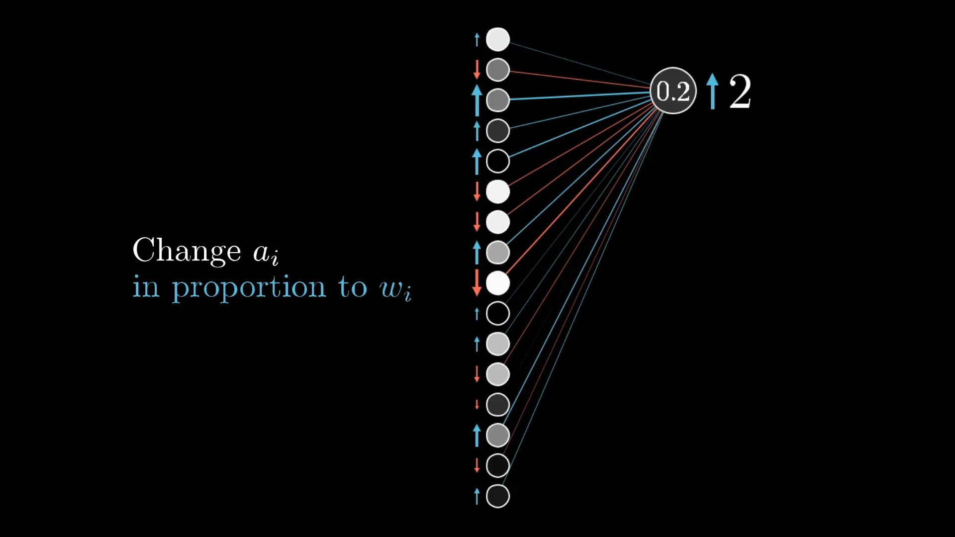
Changing the Activations
The third way to boost this neuron's activation is by tweaking the activations in the previous layer. Basically, if the neurons connected to our digit 2 neuron with positive weights light up more, and the ones connected with negative weights dim down, the digit 2 neuron will get more active.
Just like with changing the weights, the most effective changes are the ones that match up with the size of the weights themselves. So, the bigger the weight, the more impact that neuron's activation will have if you adjust it:
But here’s the catch, we can’t actually reach in and directly set these activations. The only things we really control are the weights and biases. Still, it’s useful to keep track of what changes we’d want, just like we did for the output layer.
And keep in mind, this is just what the digit 2 output neuron wants. We also want all the other output neurons to quiet down, and each of those has its own idea about what should happen to the previous layer.
So, we add up the “wishes” from all ten output neurons. Each one suggests a little nudge for the second-to-last layer, based on its own weights and how much it needs to change.
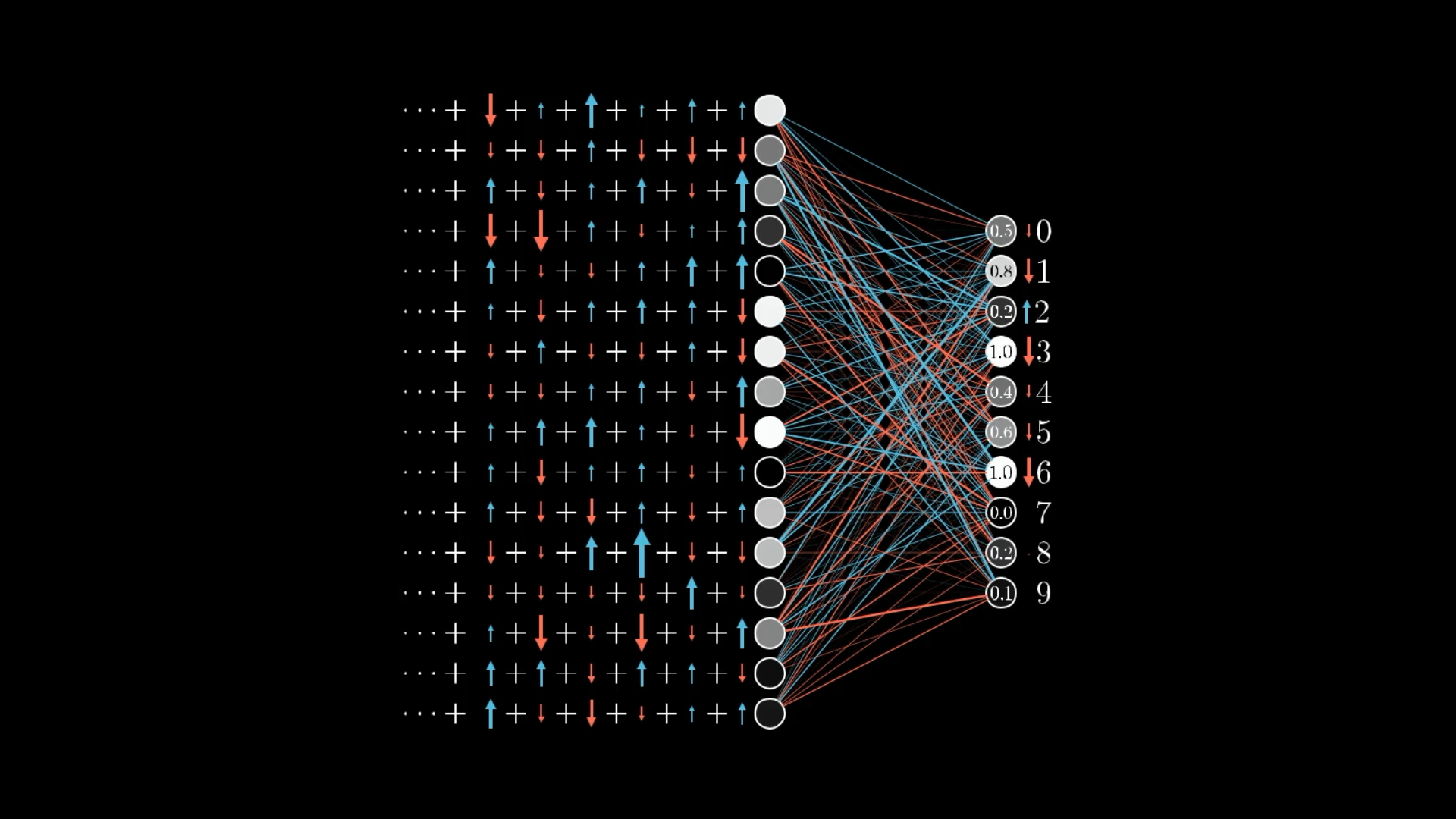
This is really what “propagating backwards” means. By combining all these desired changes, we figure out how we’d like to adjust the second-to-last layer. Then, we repeat this same process for the layers before that, working our way back through the network.
Repeating for All Training Examples
All the steps we just walked through are really just showing how a single training example wants to tweak all the different weights and biases in the network.
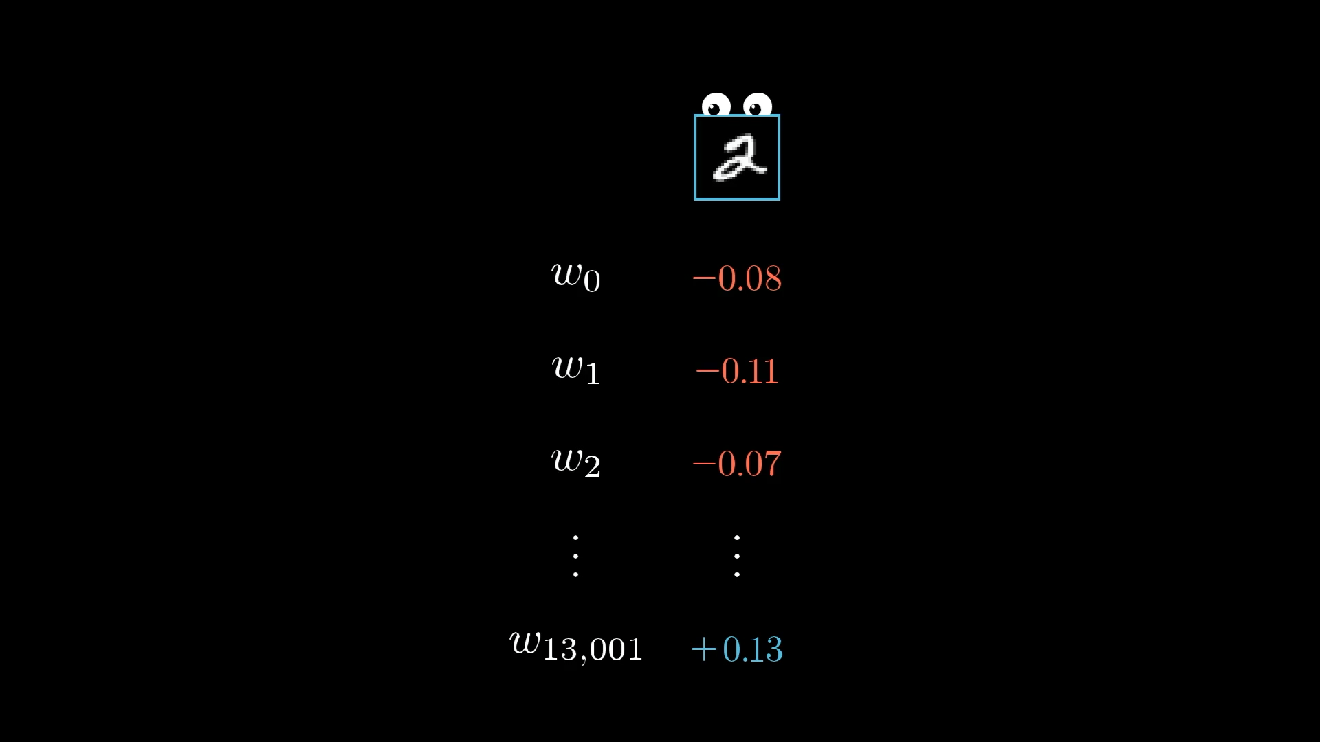
If we only paid attention to what that one image of a 2 wanted, the network would end up just trying to call everything a 2, which obviously isn’t what we want.
So, to get the bigger picture, you actually repeat this whole backpropagation process for every training example, keeping track of how each one would like to adjust the weights and biases. After that, you take all those suggestions and average them out.
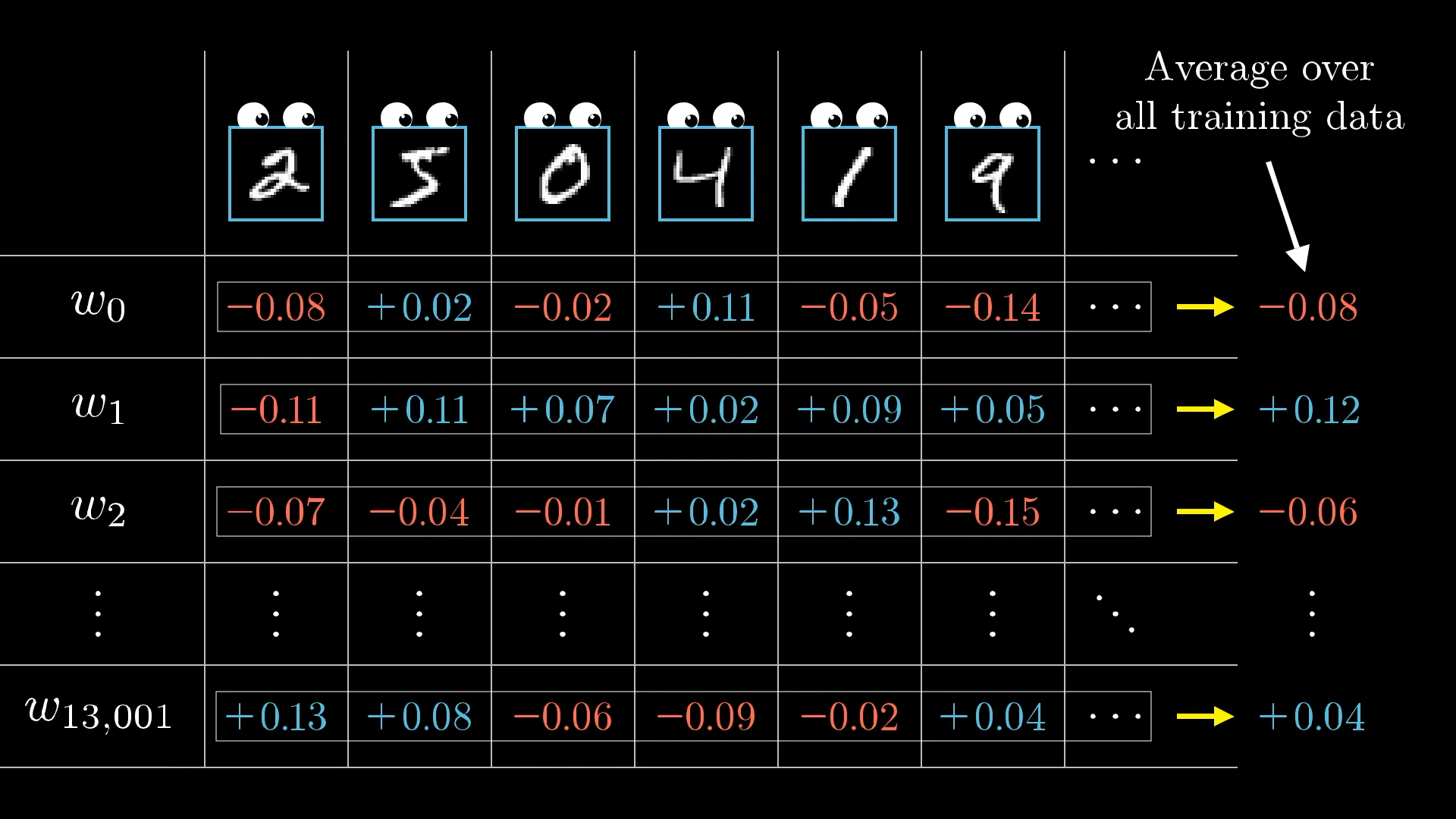
Every training example has its own idea about how the weights and biases should be changed, and how strongly. By averaging all these “wishes” together, you get the final update for each weight or bias in a single step of gradient descent.
This set of averaged nudges for each weight and bias is, in a loose sense, the negative gradient of the cost function, or at least something that points in the same direction.
I’m saying “loosely” here because I haven’t gotten into the exact maths behind these nudges. But if you get the idea of how each change works, why some are bigger than others, and how they all get combined, then you’ve basically got the core idea of what backpropagation is doing.
Stochastic Gradient Descent
When you try to add up the influence of every single training example for each step of gradient descent, it can take computers ages to get through it all. To make things faster, there’s a neat trick: rather than using the whole dataset for every step, you break your training data into smaller chunks called mini batches, maybe 100 examples in each.
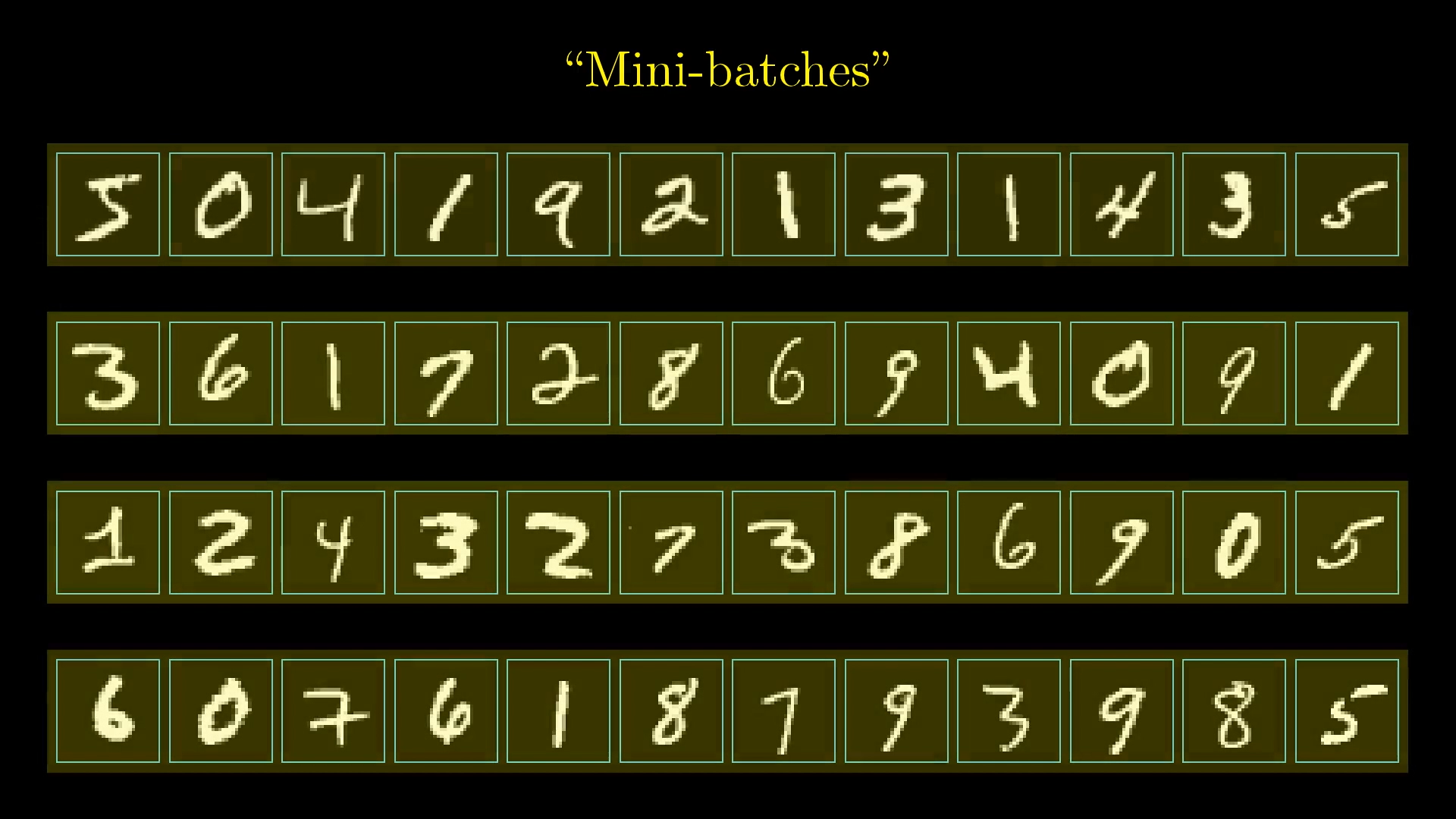
Now, instead of calculating the gradient using all your data at once, you do it for just one mini batch at a time. Sure, this doesn’t give you the exact gradient for the whole cost function, since you’re only looking at a slice of the data, but it’s a pretty good estimate. Plus, each step is way quicker, if you have 100 mini batches, each step only takes about a hundredth of the time. After you’ve gone through all the mini batches, every training example has had its say in updating the network.
This approach makes gradient descent look a bit less like someone carefully picking their way down a hill and more like someone stumbling down quickly, taking lots of fast, slightly wobbly steps. But that’s actually a good thing, because you get to the bottom much faster.
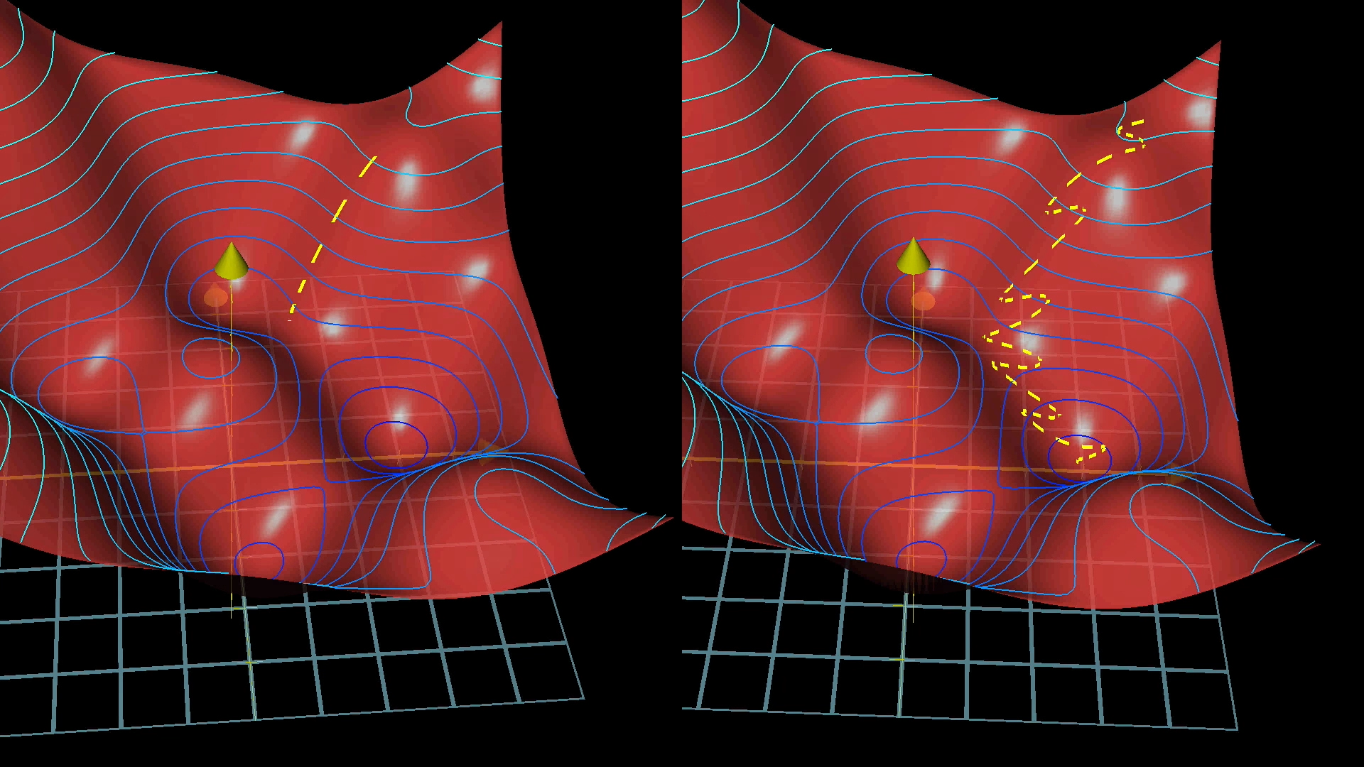
This whole method is called Stochastic Gradient Descent.
Conclusion
So, at this point, every bit of code you’d write for backpropagation lines up with something we’ve talked about, at least in a general sense. But honestly, just understanding the maths isn’t always enough, sometimes the real challenge is figuring out how to actually put it all together in code without getting lost in the details.
Implementing the Model in Python
Alright, with all that theory ammo loaded, it was time to fire it into some actual code. For this I found Michael Nielsen's book really helpful, his explanation and implementation is super clean and focuses on the essentials without any fancy bells and whistles. By the way, the full code is on my Github, give it a star if you want!
Coding the Neural Network Class
At the core of the project is a Network class. When you create an instance of this class, it sets up all the weights and biases randomly, these are just numbers that the network will tweak as it learns, and they start out following a normal (Gaussian) distribution with a mean of 0 and a variance of 1. The class has a feedforward method, which is how the network makes predictions by passing input data through each layer, applying the weights, biases, and activation function along the way. For training, it uses Stochastic Gradient Descent (SGD), which (again) is a way of gradually improving the network by looking at small batches of data at a time. The real magic happens in the backprop method, which figures out how to adjust all those weights and biases by calculating the gradients, essentially, it tells the network how to get better at its predictions. Below is a simplified version of the class, just to give you a feel for how it’s structured. If you want to see the full code, again, check out the GitHub repo.
#### Libraries
# Standard library
import random
import pickle  # Add this for saving/loading

# Third-party libraries
import numpy as np


class Network(object):

    def __init__(self, sizes):
        """The list ``sizes`` contains the number of neurons in the
        respective layers of the network.  For example, if the list
        was [2, 3, 1] then it would be a three-layer network, with the
        first layer containing 2 neurons, the second layer 3 neurons,
        and the third layer 1 neuron.  The biases and weights for the
        network are initialized randomly, using a Gaussian
        distribution with mean 0, and variance 1.  Note that the first
        layer is assumed to be an input layer, and by convention we
        won't set any biases for those neurons, since biases are only
        ever used in computing the outputs from later layers."""
        pass

    def feedforward(self, a):
        """Return the output of the network if ``a`` is input."""
        pass

    def SGD(self, training_data, epochs, mini_batch_size, eta,
            test_data=None):
        """Train the neural network using mini-batch stochastic
        gradient descent.  The ``training_data`` is a list of tuples
        ``(x, y)`` representing the training inputs and the desired
        outputs.  The other non-optional parameters are
        self-explanatory.  If ``test_data`` is provided then the
        network will be evaluated against the test data after each
        epoch, and partial progress printed out.  This is useful for
        tracking progress, but slows things down substantially."""
        pass

    def update_mini_batch(self, mini_batch, eta):
        """Update the network's weights and biases by applying
        gradient descent using backpropagation to a single mini batch.
        The ``mini_batch`` is a list of tuples ``(x, y)``, and ``eta``
        is the learning rate."""
        pass

    def backprop(self, x, y):
        """Return a tuple ``(nabla_b, nabla_w)`` representing the
        gradient for the cost function C_x.  ``nabla_b`` and
        ``nabla_w`` are layer-by-layer lists of numpy arrays, similar
        to ``self.biases`` and ``self.weights``."""
        pass

    def evaluate(self, test_data):
        """Return the number of test inputs for which the neural
        network outputs the correct result. Note that the neural
        network's output is assumed to be the index of whichever
        neuron in the final layer has the highest activation."""
        pass

    def cost_derivative(self, output_activations, y):
        """Return the vector of partial derivatives \partial C_x /
        \partial a for the output activations."""
        pass

    def save(self, filename):
        """Save weights and biases to a file."""
        pass

    @classmethod
    def load(cls, filename):
        """Load weights and biases from a file."""
        pass


#### Miscellaneous functions
def sigmoid(z):
    """The sigmoid function."""
    pass


def sigmoid_prime(z):
    """Derivative of the sigmoid function."""
    pass
Simple, right? It matches the matrix notation from earlier and the feedforward propagates activations layer by layer.
Training on MNIST Data
Loaded MNIST via a helper script mnist_loader.py. Trained a [784, 30, 10] network, 30 epochs, 10 mini batches, learning rate of 3.0. Took a few minutes on my PC.
training_data, validation_data, test_data = mnist_loader.load_data_wrapper()
net = Network([784, 30, 10])
net.SGD(training_data, 30, 10, 3.0, test_data=test_data)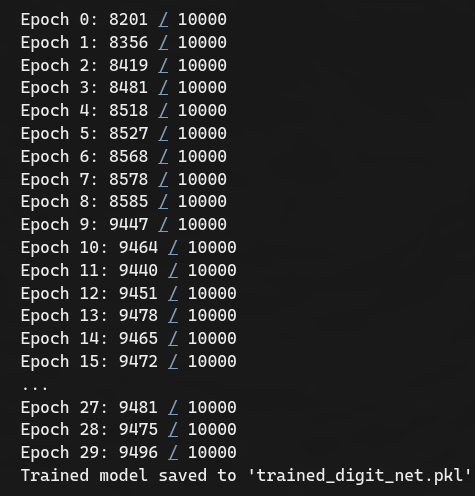
It got ~95% accuracy, bish bash bosh, the network has learned!
Also I saved it as a .pkl file for easy reload, net.save("trained_digit_net.pkl").
Testing and Saving the Model
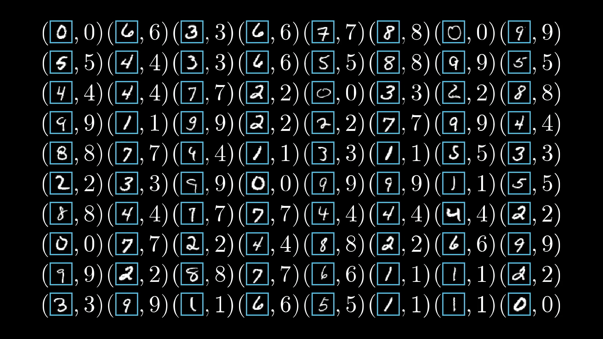
I then tested on random samples with a quick function and visualised with matplotlib to see true vs. predicted.
def test_individual_predictions(network, test_data, num_examples=5):
    indices = np.random.choice(len(test_data), num_examples)
    for i, idx in enumerate(indices):
        x, y = test_data[idx]
        prediction = np.argmax(network.feedforward(x))
        print(f"True: {y}, Predicted: {prediction}")
        plt.imshow(x.reshape(28, 28), cmap='gray')
        plt.show()

loaded_net = Network.load("trained_digit_net.pkl")
test_individual_predictions(loaded_net, test_data, 3)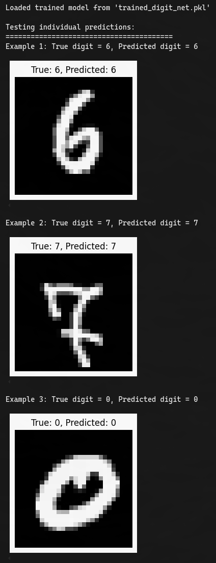
Exporting to JSON for the Web App
Now since I will be building a JS frontend app and deploying to Vercel, I cannot use python and cannot use the .pkl file for reloading, so naturally I converted the pkl to JSON. This was easy to do since the weights and biases are essentially just lists.
with open('trained_digit_net.pkl', 'rb') as f:
    data = pickle.load(f)

json_data = {
    "sizes": data["sizes"],
    "weights": data["weights"],
    "biases": data["biases"]
}

with open('trained_digit_net.json', 'w') as f:
    json.dump(json_data, f)
Building the Next.js Web App
Ok, with the model trained and exported to JSON, it's time to build the frontend bish bash bosh, a simple Next.js app where you draw on a grid and get predictions. I kept it minimal: TS, Turbopack for fast development and Shadcn for UI!
Porting the Network to TypeScript
Since I couldn’t use the Python .pkl file in JavaScript, and Vercel doesn’t let you run Python code, I had to port the feedforward part of the network to TypeScript for browser predictions. I didn’t need backpropagation here, just the forward pass. I loaded the model weights and biases from the JSON file (from earlier) in the public folder, and handled all the matrix operations with plain loops since there’s no NumPy in JS.
interface SerializedNetwork {
    sizes: number[];
    weights: number[][][];
    biases: number[][][];
}

export class Network {
    sizes: number[];
    weights: number[][][];
    biases: number[][][];

    constructor(jsonData: SerializedNetwork) {
      this.sizes = jsonData.sizes;
      this.weights = jsonData.weights;
      this.biases = jsonData.biases;
    }

    sigmoid(z: number): number {
      return 1 / (1 + Math.exp(-z));
    }

    feedforward(input: number[]): number[] {
      let activation = input.slice();
      for (let i = 0; i < this.weights.length; i++) {
        const layerWeights = this.weights[i];
        const layerBiases = this.biases[i];
        const newActivation: number[] = [];
        for (let j = 0; j < layerWeights.length; j++) {
          let z = layerBiases[j][0];
          for (let k = 0; k < layerWeights[j].length; k++) {
            z += layerWeights[j][k] * activation[k];
          }
          newActivation.push(this.sigmoid(z));
        }
        activation = newActivation;
      }
      return activation;
    }
  }

  export async function loadNetwork(): Promise<Network> {
    const res = await fetch('/trained_digit_net.json');
    const data = await res.json();
    return new Network(data);
  }
Interactive Grid Drawing Interface
I set up a 28 by 28 grid of divs with a black background, and you can draw on it in white. For smooth drawing, I used pointer and touch event handlers along with a brush effect. One tricky part was handling the difference between taps and strokes on mobile devices, so I made sure to add touch listeners with passive set to false. What that means is, by default, browsers try to optimise touch events for scrolling and other gestures, which can make drawing feel laggy or unresponsive. By setting passive to false, I can call preventDefault inside my event handler, which stops the browser from interfering and let's the drawing feel much smoother and more natural, especially on mobile devices.
const paintStroke = (fromIndex: number | null, toIndex: number) => {
    setPixels((prev) => {
      const next = prev.slice();
      const toX = toIndex % 28;
      const toY = Math.floor(toIndex / 28);
      if (fromIndex === null) {
        applyBrushAt(next, toX, toY);
        return next;
      }
      const fromX = fromIndex % 28;
      const fromY = Math.floor(fromIndex / 28);
      const dx = toX - fromX;
      const dy = toY - fromY;
      const dist = Math.max(Math.abs(dx), Math.abs(dy));
      const samples = Math.max(1, Math.ceil(dist / STEP_SIZE));
      for (let i = 0; i <= samples; i++) {
        const t = samples === 0 ? 0 : i / samples;
        const x = fromX + dx * t;
        const y = fromY + dy * t;
        applyBrushAt(next, x, y);
      }
      return next;
    });
  };

  // Keep a stable reference for native listeners
  useEffect(() => {
    paintStrokeRef.current = paintStroke;
  }, [paintStroke]);
Preprocessing Inputs for Better Accuracy
To help the model make better predictions, I preprocess the input in a few ways. First, I normalise the pixel values, which just means making sure they’re all between 0 and 1, so the network isn’t thrown off by different brightness levels. Then, I centre the digit in the grid, so it doesn’t matter if you draw your number off to one side or the other (which throws the model off). I also scale the digit a bit, which helps because people draw numbers in all sorts of sizes, and resizing them to fit a similar area makes things more consistent for the model.
const preprocess = (src: number[]): number[] => {
    const threshold = 0.1;
    let minX = 28, minY = 28, maxX = -1, maxY = -1;
    for (let y = 0; y < 28; y++) {
      for (let x = 0; x < 28; x++) {
        const v = src[y * 28 + x];
        if (v > threshold) {
          if (x < minX) minX = x;
          if (y < minY) minY = y;
          if (x > maxX) maxX = x;
          if (y > maxY) maxY = y;
        }
      }
    }
    if (maxX < 0) {
      return new Array(28 * 28).fill(0);
    }

    const width = maxX - minX + 1;
    const height = maxY - minY + 1;
    const scale = 0.8; // slight zoom out
    const newWidth = Math.max(1, Math.floor(width * scale));
    const newHeight = Math.max(1, Math.floor(height * scale));
    const centreX = Math.floor((28 - newWidth) / 2);
    const centreY = Math.floor((28 - newHeight) / 2);

    const dst = new Array(28 * 28).fill(0);
    for (let ny = 0; ny < newHeight; ny++) {
      for (let nx = 0; nx < newWidth; nx++) {
        const ox = Math.min(27, Math.max(0, minX + Math.floor(nx / scale)));
        const oy = Math.min(27, Math.max(0, minY + Math.floor(ny / scale)));
        const oldIdx = oy * 28 + ox;
        const newX = centreX + nx;
        const newY = centreY + ny;
        const newIdx = newY * 28 + newX;
        dst[newIdx] = Math.max(dst[newIdx], src[oldIdx]);
      }
    }
    return dst;
  };
Deployment on Vercel
Once I finished the project, I pushed the code to GitHub, and Vercel took care of the deployment automatically, which was super convenient. I also set up some basic analytics to keep track of how people are using the app, and that was both free and really easy to do. If you want to try it out yourself, you can check out the live version here: https://handwritten-digit-recogniser.vercel.app/. When you’re testing, try drawing your digit as large as possible so it fills up most of the grid, this helps the model make the most accurate prediction.
Challenges and Learnings
The main challenge I ran into was with mobile compatibility. On desktop, everything worked perfectly, and even when I used the Chrome dev tools to emulate a mobile device, drawing strokes was fine. But as soon as I pushed the app to Vercel and tried it on my actual phone, I couldn’t draw a proper stroke at all—it would just put a dot wherever I tried to draw a stroke, instead of letting me draw a line. Since I needed this to work for a live demo at work, I had to dig in and figure out what was going on. After a bit of tinkering (which I explained above), I managed to fix it, but it definitely took some trial and error.
Another funny thing is that I kept pushing to Vercel every time I got stuck on the bug, totally forgetting that I could just access the app from my phone using my computer’s IP address while it was running locally on my network. Would’ve saved me a bit of time, but hey, you live and learn.
On the learning side, diving into the theory behind all this really helped demystify machine learning for me. It’s not magic, it’s just a lot of optimisation and calculus. I also didn’t realise how important preprocessing the user input was until I ran into issues, at first, the model wasn’t recognising any of my numbers, which was kind of hilarious. But that kind of makes sense since my network is super basic. I was also originally using a canvas to draw instead of the current div setup, so that made a difference too.
The End
So, bish bash bosh, I went from scribbled notes to a working app, and it was a pretty cool journey. If you have any feedback, feel free to reach out to me wherever you can find me (links below). And if you end up checking out the source code, maybe give it a star if you feel like it.
Thanks for reading!